Quantitative Trading

Financial engineers are accustomed to borrowing techniques from scientists in other fields (e.g. genetic algorithms), but rarely does the borrowing go the other way. It is therefore surprising to hear about this paper on a possible mechanism for evolution due to natural selection which is inspired by universal capital allocation algorithms.

A capital allocation algorithm attempts to optimize the allocation of capital to stocks in a portfolio. An allocation algorithm is called universal if it results in a net worth that is "similar" to that generated by the best constant-rebalanced portfolio with fixed weightings over time (denoted CBAL* below), chosen in hindsight. "Similar" here means that the net worth does not diverge exponentially. (For a precise definition, see this very readable paper by Borodin, et al. H/t: Vladimir P.)

Previously, I know only of one such universal trading algorithm - the Universal Portfolio invented by Thomas Cover, which I have described before. But here is another one that has proven to be universal: the exceedingly simple EG algorithm.

The EG ("Exponentiated Gradient") algorithm is an example of a capital allocation rule using "multiplicative updates": the new capital allocated to a stock is proportional to its current capital multiplied by a factor. This factor is an exponential function of the return of the stock in the last period. This algorithm is both greedy and conservative: greedy because it always allocates more capital to the stock that did well most recently; conservative because there is a penalty for changing the allocation too drastically from one period to the next. This multiplicative update rule is the one proposed as a model for evolution by natural selection.

The computational advantage of EG over the Universal Portfolio is obvious: the latter requires a weighted average over all possible allocations at every step, while the former needs only know the allocation and returns for the most recent period. But does this EG algorithm actually generate good returns in practice? I tested it two ways:

1) Allocate between cash (with 2% per annum interest) and SPY.
2) Allocate among SP500 stocks.

In both cases, the only free parameter of the model is a number called the "learning rate" η, which determines how fast the allocation can change from one period to the next. It is generally found that η=0.01 is optimal, which we adopted. Also, we disallow short positions in this study.

The benchmarks for comparison for 1) are, using the notations of the Borodin paper,

a) the buy-and-hold SPY portfolio BAH, and
b) the best constant-rebalanced portfolio with fixed allocations in hindsight CBAL*.

The benchmarks for comparison for 2) are

a) a constant rebalanced portfolio of SP500 stocks with equal allocations U-CBAL,
b) a portfolio with 100% allocation to the best stock chosen in hindsight BEST1, and
c) CBAL*.

To find CBAL* for a SP500 portfolio, I used Matlab Optimization Toolbox's constrained optimization function fmincon.

There is also the issue of SP500 index reconstitution. It is complicated to handle the addition and deletion of stocks in the index within a constrained optimization function. So I opted for the shortcut of using a subset of stocks that were in SP500 from 2007 to 2013, tolerating the presence of surivorship bias. There are only 346 such stocks.

The result for 1) (cash vs SPY) is that the CAGR (compound annualized growth rate) of EG is slightly lower than BAH (4% vs 5%). It turns out that BAH and CBAL* are the same: it was best to allocate 100% to SPY during 2007-2013, an unsurprising recommendation in hindsight.

The result for 2) is that the CAGR of EG is higher than the equal-weight portfolio (0.5% vs 0.2%). But both these numbers are much lower than that of BEST1 (39.58%), which is almost the same as that of CBAL* (39.92%). (Can you guess which stock in the current SP500 generated the highest CAGR? The answer, to be revealed below*, will surprise you!)

We were promised that the EG algorithm will perform "similarly" to CBAL*, so why does it underperform so miserably? Remember that similarity here just means that the divergence is sub-exponential: but even a polynomial divergence can in practice be substantial! This seems to be a universal problem with universal algorithms of asset allocation: I have never found any that actually achieves significant returns in the short span of a few years. Maybe we will find more interesting results with higher frequency data.

So given the underwhelming performance of EG, why am I writing about this algorithm, aside from its interesting connection with biological evolution? That's because it serves as a setup for another, non-universal, portfolio allocation scheme, as well as a way to optimize parameters for trading strategies in general: both topics for another time

===
Workshops Update:

My next online workshop will be on Mean Reversion Strategies, August 26-28. This and the Quantitative Momentum workshops will also be conducted live at Nanyang Technological University in Singapore, September 18-21.

===
Do follow me @chanep on Twitter, as I often post links to interesting articles there.

===
*The SP500 stock that generated the highest return from 2007-2013 is AMZN.

In my book, I described a very simple and elegant formula for determining the optimal asset allocation among N assets:

F=C^-1*M (1)

where F is a Nx1 vector indicating the fraction of the equity to be allocated to each asset, C is the covariance matrix, and M is the mean vector for the excess returns of these assets. Note that these "assets" can in fact be "trading strategies" or "portfolios" themselves. If these are in fact real assets that incur a carry (financing) cost, then excess returns are returns minus the risk-free rate.

Notice that these fractions, or weights as they are usually called, are not normalized - they don't necessarily add up to 1. This means that F not only determines the allocation of the total equity among N assets, but it also determines the overall optimal leverage to be used. The sum of the absolute value of components of F divided by the total equity is in fact the overall leverage. Thus is the beauty of Kelly formula: optimal allocation and optimal leverage in one simple formula, which is supposed to maximize the compounded growth rate of one's equity (or equivalently the equity at the end of many periods).

However, most students of finance are not taught Kelly portfolio optimization. They are taught Markowitz mean-variance portfolio optimization. In particular, they are taught that there is a portfolio called the tangency portfolio which lies on the efficient frontier (the set of portfolios with minimum variance consistent with a certain expected return) and which maximizes the Sharpe ratio. Left unsaid are

What's so good about this tangency portfolio?
What's the real benefit of maximizing the Sharpe ratio?
Is this tangency portfolio the same as the one recommended by Kelly optimal allocation?

I want to answer these questions here, and provide a connection between Kelly and Markowitz portfolio optimization.

According to Kelly and Ed Thorp (and explained in my book), F above not only maximizes the compounded growth rate, but it also maximizes the Sharpe ratio. Put another way: the maximum growth rate is achieved when the Sharpe ratio is maximized. Hence we see why the tangency portfolio is so important. And in fact, the tangency portfolio is the same as the Kelly optimal portfolio F, except for that fact that the tangency portfolio is assumed to be normalized and has a leverage of 1 whereas F goes one step further and determines the optimal leverage for us. Otherwise, the percent allocation of an asset in both are the same (assuming that we haven't imposed additional constraints in the optimization problem). How do we prove this?

The usual way Markowitz portfolio optimization is taught is by setting up a constrained quadratic optimization problem - quadratic because we want to optimize the portfolio variance which is a quadratic function of the weights of the underlying assets - and proceed to use a numerical quadratic programming (QP) program to solve this and then further maximize the Sharpe ratio to find the tangency portfolio. But this is unnecessarily tedious and actually obscures the elegant formula for F shown above. Instead, we can proceed by applying Lagrange multipliers to the following optimization problem (see http://faculty.washington.edu/ezivot/econ424/portfolioTheoryMatrix.pdf for a similar treatment):

Maximize Sharpe ratio = F^T*M/(F^T*C*F)^1/2(2)

subject to constraint F^T*1=1 (3)

(to emphasize that the 1 on the left hand side is a column vector of one's, I used bold face.)

So we should maximize the following unconstrained quantity with respect to the weights F_iof each asset i and the Lagrange multiplier λ:

F^T*M/(F^T*C*F)^{1/2 -}λ(F^T*1-1) (4)

But taking the partial derivatives of this fraction with a square root in the denominator is unwieldy. So equivalently, we can maximize the logarithm of the Sharpe ratio subject to the same constraint. Thus we can take the partial derivatives of

log(F^T*M)-(1/2)*log(F^T*C*F)^-λ(F^T*1-1) (5)

with respect to F_i. Setting each component i to zero gives the matrix equation

(1/F^T*M)M-(1/F^T*C*F)C*F=λ1 (6)

Multiplying the whole equation by F^Ton the right gives

(1/F^T*M)F^T*M-(1/F^T*C*F)F^T*C*F=λF^T*1 (7)

Remembering the constraint, we recognize the right hand side as just λ. The left hand side comes out to be exactly zero, which means that λ is zero. A Lagrange multiplier that turns out to be zero means that the constraint won't affect the solution of the optimization problem up to a proportionality constant. This is satisfying since we know that if we apply an equal leverage on all the assets, the maximum Sharpe ratio should be unaffected. So we are left with the matrix equation for the solution of the optimal F:

C*F=(F^T*C*F/F^T*M)M (8)

If you know how to solve this for F using matrix algebra, I would like to hear from you. But let's try an ansatz F=C^-1*M as in (1). The left hand side of (8) becomes M, the right hand side becomes (F^T*M/F^T*M)M = M as well. So the ansatz works, and the solution is in fact (1), up to a proportionality constant. To satisfy the normalization constraint (3), we can write

F=C^-1*M / (1^T*C^-1*M) (9)

So there, the tangency portfolio is the same as the Kelly optimal portfolio, up to a normalization constant, and without telling us what the optimal leverage is.

===

Workshop Update:

Based on popular demand, I have revised the dates for my online Mean Reversion Strategies workshop to be August 27-29.

===

Follow me @chanep on Twitter.

Many traders who use technical analysis favor the Moving Average Crossover as a momentum indicator. They compute the short-term minus the long-term moving averages of prices, and go long if this indicator just turns positive, or go short if it turns negative. This seems intuitive enough. What isn't obvious, however, is that MA Crossover is nothing more than an estimate of the recent average compound return.

But just when you might be tempted to ditch this indicator in favor of the average compound return, it can be shown that the MA Crossover is also a triangle filter on the 1-period returns. (A triangle filter in signal processing is a set of weights imposed on a time series that increases linearly with time up to some point, and then decreases linearly with time up to the present time. See the diagram at the end of this article.) Why is this interpretation interesting? That's because it leads us to consider other, more sophisticated filters (such as the least square, Kalman, or wavelet filters) as possible momentum indicators. In collaboration with my former workshop participant Alex W. who was inspired by this paper by Bruder et. al., we present the derivations below.

===

First, note that we will compute the moving average of log prices y, not raw prices. There is of course no loss or gain in information going from prices to log prices, but it will make our analysis possible. (The exact time of the crossover, though, will depend on whether we use prices or log prices.) If we write MA(t, n1) to denote the moving average of n1 log prices ending at time t, then the moving average crossover is MA(t, n1)-MA(t, n2), assuming n1< n2. By definition,

MA(t, n1)=(y(t)+y(t-1)+...+y(t-n1+1))/n1
MA(t, n2)=(y(t)+y(t-1)+...+y(t-n1+1)+y(t-n1)+...+y(t-n2+1)/n2

MA(t, n1)-MA(t, n2)
=[(n2-n1)/(n1*n2)] *[y(t)+y(t-1)+...+y(t-n1+1)] - (1/n2)*[y(t-n1)+...+y(t-n2+1)]
=[(n2-n1)/n2] *MA(t, n1)-[(n2-n1)/n2]*MA(t-n1, n2-n1)
=[(n2-n1)/n2]*[MA(t, n1)-MA(t-n1, n2-n1)]

If we interpret MA(t, n1) as an approximation of the log price at the midpoint (n1-1)/2 of the time interval [t-n1+1, t], and MA(t-n1, n2-n1) as an approximation of the log price at the midpoint (n2-n1-1)/2 of the time interval [t-n1, t-(n2-n1)], then [MA(t, n1)-MA(t-n1, n2-n1)] is an approximation of the total return over a time period of n2/2. If we write this total return as an average compound growth rate r multiplied by the period n2/2, we get

MA(t, n1)-MA(t, n2) ≈ [(n2-n1)/n2]*(n2/2)*r

r ≈ [2/(n2-n1)]*[MA(t, n1)-MA(t, n2)]

as shown in Equation 4 of the paper cited above. (Note the roles of n1 and n2 are reversed in that paper.)

===

Next, we will show why the MA crossover is also a triangle filter on 1-period returns. Simplifying notation by fixing t to be 0,

MA(t=0, n1)
=(y(0)+y(-1)+...+y(-n1+1))/n1
=(1/n1)*[(y(0)-y(-1))+2(y(-1)-y(-2))+...+n1*(y(-n1+1)-y(-n1))]+y(-n1)

Writing the returns from t-1 to t as R(t), this becomes

MA(t=0, n1)=(1/n1)*[R(0)+2*R(-1)+...+n1*R(-n1+1)]+y(-n1)

Similarly,

MA(t=0, n2)=(1/n2)*[R(0)+2*R(-1)+...+n2*R(-n2+1)]+y(-n2)

So MA(0, n1)-MA(0, n2)
=(1/n1-1/n2)*[R(0)+2*R(-1)+...+n1*R(-n1+1)]
-(1/n2)*[(n1+1)*R(-n1)+(n1+2)*R(-n1-1)+...+n2*R(-n2+1)]
+y(-n1)-y(-n2)

Note that the last line above is just the total cumulative return from -n2 to -n1, which can be written as

y(-n1)-y(-n2)=R(-n1)+R(-n1-1)+...+R(-n2+1)

Hence we can absorb that into the expression prior to that

MA(0, n1)-MA(0, n2)
=(1/n1-1/n2)*[R(0)+2*R(-1)+...+n1*R(-n1+1)]
-(1/n2)*[(n1+1-n2)*R(-n1)+(n1+2-n2)*R(-n1-1)+...+(-1)*R(-n2+2)]
=(1/n1-1/n2)*[R(0)+2*R(-1)+...+n1*R(-n1+1)]
+(1/n2)*[(n2-n1-1)*R(-n1)+(n2-n1-2)*R(-n1-1)+...+R(-n2+2)]

We can see the coefficients of R's from t=-n2+2 to -n1 form the left side of an triangle with positive slope, and those from t=-n1+1 to 0 form the right side of the triangle with negative slope. The plot (click to enlarge) below shows the coefficients as a function of time, with n2=10, n1=7, and current time as t=0. The right-most point is the weight for R(0): the return from t=-1 to 0.

Q.E.D. Now I hope you are ready to move on to a wavelet filter!

P.S. It is wonderful to be able to check the correctness of messy algebra like those above with a simple Matlab program!

===

New Service Announcement

Our firm QTS Capital Management has recently launched a FX Managed Accounts program. It uses one of the mean-reverting strategies we have been trading successfully in our fund for the last three years, and is still going strong despite the low volatility in the markets. The benefits of a managed account are that clients retain full ownership and control of their funds at all times, and they can decide what level of leverage they are comfortable with. Unlike certain offshore FX operators, QTS is a CPO/CTA regulated by the National Futures Association and the Commodity Futures Trading Commission.

===

Workshops Update

Readers may be interested in my next workshop series to be held in London, November 3-7. Please follow the link at the bottom of this page for information.

===
Follow me on Twitter: @chanep

By Roger Hunter

I am a quant researcher and developer for QTS Partners, a commodity pool Ernie (author of this blog) founded in 2011. I help Ernie develop and implement several strategies in the pool and various separate accounts. I wrote this article to give insights into a very important part of our strategy development process: the selection of data sources.

Our main research focus is on strategies that monitor execution in milliseconds and that hold for seconds through several days. For example, a strategy that trades more than one currency pair simultaneously must ensure that several executions take place at the right price and within a very short time. Backtesting requires high quality historical intraday quote and trade, preferably tick data for testing. Our initial focus was futures and after looking at various vendors for the tick data quality and quantity we needed, we chose Nanex data which is aggregated at 25ms. This means, for example, that aggressor flags are not available. We purchased several years of futures data and set to work.

Earlier this year we needed to update our data and discovered that Nanex prices had increased significantly. We also needed quotes and trades, and data for more asset classes including US equities and options.

We looked at TickData.com which has good data but is very expensive and you pay up-front per symbol. There are other services like Barchartondemand.com and XIgnite.com where you pay based on your monthly usage (number of data requests made) which is a model we do not like. We ended up choosing QuantGo.com, where you have unlimited access to years of global tick or bar data for a fixed monthly subscription fee per data service.

On QuantGo, you get computer instances in your own secure and private cloud built on Amazon AWS with on-demand access to a wide range of global intraday tick or bar data from multiple data vendors. Since you own and manage the computer instances you can choose any operating system, install any software, access the internet or import your own data. With QuantGo the original vendor data must remain in the cloud but you can download your results, this allows QuantGo to rent access to years of data at affordable monthly prices.

All of the data we have used so far is from AlgoSeek (one of QuantGo’s data vendors). This data is survivorship bias-free and is exactly as provided by the exchanges at the time. Futures quotes and trades download very quickly on the system. I am testing options strategies, which is challenging due to the size of the data. The data is downloaded in highly compressed form which is then expanded (by QuantGo) to a somewhat verbose text form. Before the price split, a day of option quotes and trades for AAPL was typically 100GB in this form. Here is a data sample from the full Options (OPRA) data:

Timestamp, EventType, Ticker, OptionDetail, Price, Quantity, Exchange, Conditions
08:30:02.493, NO_QUOTE BID NB, LLEN, PUT at 7.0000 on 2013-12-21, 0.0000, 0, BATS, F
08:30:02.493, NO_QUOTE ASK, LLEN, CALL at 7.0000 on 2013-12-21, 0.0000, 0, BATS, F
09:30:00.500, ROTATION ASK, LLEN, PUT at 2.0000 on 2013-07-20, 0.2500, 15, ARCA, R
09:30:00.500, ROTATION BID, LLEN, PUT at 2.0000 on 2013-07-20, 0.0000, 0, ARCA, R
09:30:00.507, FIRM_QUOTE ASK NB, LLEN, PUT at 5.0000 on 2013-08-17, 5.0000, 7, BATS, A
09:30:00.508, FIRM_QUOTE BID NB, LLEN, PUT at 6.0000 on 2013-08-17, 0.2000, 7, BATS, A

These I convert to a more compact format, and filter out lines we don't need (e.g. NO_QUOTE, non-firm, etc.)

The quality of the AlgoSeek data seems to be high. One test I have performed is to record live data and compare it with AlgoSeek. This is possible because the AlgoSeek historical data is now updated daily, and is one day behind for all except options, which varies from two days to five (they are striving for two, but the process involves uploading all options data to special servers --- a significant task). Another test is done using OptionNET Explorer (ONE). ONE data is at 5-minute intervals and the software displays midpoints only. However, by executing historical trades, you can see the bid and ask values for options at these 5-minute boundaries. I have checked 20 of these against the AlgoSeek data and found exact agreement in every case. In any event, you are free to contact the data vendors directly to learn more about their products. The final test of data quality (and of our market model) is the comparison of live trading results (at one contract/spread level) with backtests over the same period.

The data offerings have recently expanded dramatically with more data partners and now include historical data from (QuantGo claims) "every exchange in the world". I haven't verified this, but the addition of elementized, tagged and scored news from Acquire Media, for example, will allow us to backtest strategies of the type discussed in Ernie's latest book.

So far, we like the system. For us, the positives are:

1. Affordable Prices. The reason that the price has been kept relatively low is that original vendor data must be kept and used in the QuantGo cloud. For example, to access years of US data we have been paying
Five years of US Equities Trades and Quotes (“TAQ”) is $250 per month
Five years of US Equities 5 minute Bars $75 per month
Three Years of US Options 1 minute bars $100 per month.
Three Year of CME, CBOT, NYMEX Futures Trades and Quotes $250 per month

2. Free Sample Data. Each data service has free demo data which is actual real historical data where I can select data from the demo date range. This allowed me to view and work with the data before subscribing.

3. One API. I have one API to access different data vendors. QuantGo gives me a java GUI, python CLI and various libraries (R, Matlab, Java).

4. On-Demand. The ability to select the data we want "on demand" via a subscription from a website console at any time. You can select data for any symbol and for just a day or for several years.

5. Platform not proprietary. We can use any operating system or software with the data as it is being downloaded to virtual computers we fully control and manage.

Because all this is done in the cloud, we have to pay for our cloud computer usage as well. While cloud usage is continuing to drop rapidly in price it is still a variable cost and it needs to monitored. QuantGo does provide close to real-time billing estimates and alarms you can preset at dollar values.

I was at first skeptical of the restriction of not being able to download the data vendor’s tick or bar data, but so far this hasn't been an issue as in practice we only need the results and our derived data sets. I'm told that if you want to buy the data for your own computers, you can negotiate directly with the individual data vendor and will get a discount if you have been using it for a while on QuantGo.

As we use the windows operating system we access our cloud computers with Remote Desktop and there have been some latency issues, but these are tolerable. On the other hand, it is a big advantage to be able to start with a relatively small virtual machine for initial coding and debugging, then "dial up" a much larger machine (or group of machines) when you want to run many compute and data intensive backtests. While QuantGo is recently launched and is not perfect, it does open up the world of the highest institutional quality data to those of us who do not have the data budget of a Renaissance Technologies or D.E. Shaw.

===
Industry Update
(No endorsement of companies or products is implied by our mention.)

A new site for jobs in finance was recently launched: www.financejobs.co.
A new software package Geode by Georgica Software can backtest tick data, and comes with a fairly rudimentary fill simulator.
Quantopian.com now incorporates a new IPython based research environment that allows interactive data analysis using minute level pricing data in Python.

===

Workshops Update

My next online Quantitative Momentum Strategies workshop will be held on December 2-4. Any reader interested in futures trading in general would benefit from this course.

===
Managed Account Program Update

Our FX Managed Account program had an unusually profitable month in October.

===
Follow me on Twitter: @chanep

By Yang Gao

Estimize is an online-community utilizing 'wisdom of crowds' to offer intelligence about market. It contains a wide range of crowd-sourced estimates from over 4,500 buy-side, sell-side and individual analysts. Studies (from Deustche Bank and Rice University among others) show estimates from Estimize are more accurate than estimates from traditional sell-side analysts.

The first strategy we tested is a mean reversion strategy developed by the quantitative research team from Deltix using Estimize’s data. This strategy is based on the idea that post-earning-announcement prices typically revert from the short-term trend driven by the more recent Estimize estimates just before the announcement. We backtested this strategy with S&P100 over the period between 2012/01/01 and 2013/12/31. (Even though Estimize has 2014 data, we do not have the corresponding survivorship-bias-free price data from the Center for Research in Securities Prices that includes the closing bid and ask prices.) With 5bp one-way transaction cost, we found that the backtest shows a Sharpe ratio of 0.8 and an average annual return of 6%. The following figure is the cumulative P&L of the strategy based on $1 per stock position.

Cumulative P&L of Deltix Mean Reversion Strategy with Estimize

It surprised us that a mean-reverting instead of a momentum strategy was used in conjunction with Estimize data, since earnings estimates and announcements typically generate price momentum. In order to show that this return is really driven by the information in Estimize and not simply due to price reversal, we provide a benchmark mean-reverting strategy that uses prices alone to generate signal:

1. Find long period T and short period T_s, where T is average period of the reporting of all the quarterly estimates and T_s is average period of the reporting of the latest 20% of all estimates.
2. Calculate stock return R over T and Rs over T_s, and let delta = R - Rs
3. Buy stocks with delta > 0 at close before an earnings announcement and exit the positions next morning at the open after the announcement.
4. Sell stocks with delta < 0 at close before an earnings announcement and exit the positions next morning at the open after the announcement.
5. Hedge net exposure with SPY during the entire holding period.

This benchmark shows no significant positive return and so it does seem that there is useful information in the Estimize data captured by Deltix’s mean-reversion strategy.

Next, we compare the traditional earnings estimates from I/B/E/S gathered from sell-side Wall Street analysts to the crowd-sourced Estimize estimates. Backtest showed the same Deltix mean reversion strategy described above but using I/B/E/S estimates gave negative return over the same S&P100 universe and over the same 2012-2013 period, again supporting the thesis that Estimize estimates may be superior.

Since Deltix's mean reversion strategy gives negative returns on I/B/E/S data, it is natural to see if a momentum strategy would work instead: if the short-term average estimate is higher than the long-term average estimate (i.e. analogous to delta < 0 above), we expect the price to move up and vice verse.

The backtest result of this momentum strategy over the same universe and time period is quite promising: with 5bp transaction cost, the Sharpe ratio = 1.5 and average annual return = 11%. The following figure is the daily P&L of the strategy based on $1 per stock position

Cumulative P&L of momentum Strategy with I/B/E/S

We tried the same momentum strategy using Estimize data over 2012-2013, and it generated negative returns this time. This is not surprising since we found earlier that the mean reversion strategy using Estimize data generated positive returns.

We proceeded to backtest this momentum strategy over the S&P100 using out-of-sample I/B/E/S data between 2010 and 2012, and unfortunately the strategy failed there too. The following figure is the daily P&L of the strategy from 2010-2014.

Cumulative P&L of momentum Strategy with I/B/E/S

So how would Deltix’s mean-reversion strategy with Estimize data work over this out-of-sample period? Unfortunately, we won’t know because Estimize didn't start collecting data until the end of 2011. The following table is a summary on the annual returns comparing different strategies using different data sets and periods.

Strategies	Mean-Reversion	Momentum
Estimize (2012.01-2013.12)	6%	-9%
I/B/E/S (2012.01-2013.12)	-17%	11%
I/B/E/S (2010.01-2011.12)	1.8%	-6.4%

As a result, we cannot conclude that Estimize data is consistently better than I/B/E/S data in terms of generating alpha: it depends on the strategy deployed. We also cannot decide which strategy – mean-reversion or momentum – is consistently better: it depends on the time period and the data used. The only conclusion we can reach is that the short duration of the Estimize data coupled with our lack of proper price data in 2014 means that we cannot have a statistically significant backtest. This state of inconclusiveness will of course be cured in time.

_________

Yang Gao, Ph.D., is a research intern at QTS Capital Management, LLC.

===

Industry Update

(No endorsement of companies or products is implied by our mention.)

There is a good discussion comparing Quantconnect to Quantopian here.
For FX traders, Rizm offers a comparable service as Quantconnect and Quantopian as it is directly connected to FXCM.
Quantopian now offers free fundamental data from MorningStar. Also, check out their Quantopian Managers Program where you can compete to manage real money.

===

Workshop Update

Our next online workshop will be Millisecond Frequency Trading on March 25-26. It is for traders who are interested in intraday trading (even if not at millisecond frequency) and who want to defend against certain HFT tactics.

===

Managed Account Program Update

Our FX Managed Account program had a strong finish in 2014, with annual net return of 69.86%.

===

Follow me on Twitter: @chanep

In our drive to extract alphas from a variety of non-price data, we came across this old-fashioned source: Commitments of Traders (COT) on futures. This indicator is well-known to futures traders since 1923 (see www.cmegroup.com/education/files/COT_FBD_Update_2012-4-26.pdf), but there are often persistent patterns (risk factors?) in the markets that refuse to be arbitraged away. It is worth another look, especially since the data has become richer over the years.

First, some facts about COT:
1) CFTC collects the reports of the number of long and short futures and options contracts ("open interest") held by different types of firms by Tuesdays, and reports them every Friday by 4:30 CT.
2) Options positions are added to COT as if they were futures but adjusted by their deltas.
3) COT are then broken down into contracts held by different types of firms. The most familiar types are "Commercial" (e.g. an ethanol plant) and "Non-Commercial" (i.e. speculators).
4) Other types are "Spreaders" who hold calendar spreads, "Index traders", "Money Managers", etc. There are 9 mutually exclusive types in total.

Since we only have historical COT data from csidata.com, and they do not collect data on all these types, we have to restrict our present analysis only to Commercial and Non-Commercial. Also, beware that csidata tags a COT report by its Tuesday data collection date. As noted above, that information is unactionable until the following Sunday evening when the market re-opens.

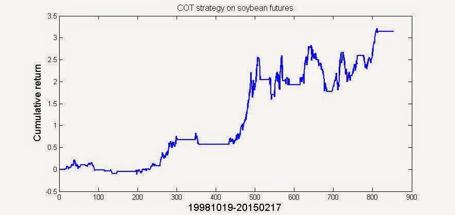
A simple strategy would be to compute the ratio of long vs short COT for Non-Commercial traders. We buy the front contract when this ratio is equal to or greater than 3, exiting when the ratio drops to or below 1. We short the front contract when this ratio is equal to or less than 1/3, exiting when the ratio rises to or above 1. Hence this is a momentum strategy: we trade in the same direction as the speculators did. As most profitable futures traders are momentum traders, it would not be surprising this strategy could be profitable.

Over the period from 1999 to 2014, applying this strategy on CME soybean futures returns about 9% per annum, though its best period seems to be behind us already. I have plotted the cumulative returns below (click to enlarge).

I have applied this strategy to a few other agricultural commodities, but it doesn't seem to work on them. It is therefore quite possible that the positive result on soybeans is a fluke. Also, it is very unsatisfactory that we do not have data on the Money Managers (which include the all important CPOs and CTAs), since they would likely to be an important source of alpha. Of course, we can go directly to the cftc.gov, download all the historical reports in .xls format, and compile the data ourselves. But that is a project for another day.

===

My Upcoming Talks and Workshops

3/14:"Beware of Low Frequency Data" at QuantCon 2015, New York.

3/22-

\infty

: "Algorithmic Trading of Bitcoins" pre-recorded online workshop.

3/24-25: "Millisecond Frequency Trading" live online workshop.

5/13-14: "Mean Reversion Strategies", "AI techniques in Trading" and "Portfolio Optimization" at Q-Trade Bootcamp 2015, Milan, Italy.

5/18-22: "Statistical Arbitrage", 'Quantitative Momentum", and "Millisecond Frequency Trading", London, UK.

===

Managed Account Program Update

Our FX Managed Account program has a net return of +7.68% in February (YTD: +8.06%).

===

Follow me on Twitter: @chanep

(This post is based on the talk of the same title I gave at Quantopian's NYC conference which commenced at 3.14.15 9:26:54. Do these numbers remind you of something?)

A correct backtest of a trading strategy requires accurate historical data. This isn't controversial. Historical data that is full of errors will generate fictitious profits for mean-reverting strategies, since noise in prices is mean-reverting. However, what is lesser known is how perfectly accurate capture of historical prices, if done in a sub-optimal way, can still lead to dangerously inflated backtest results. I will illustrate this with three simple strategies.

CEF Premum Reversion

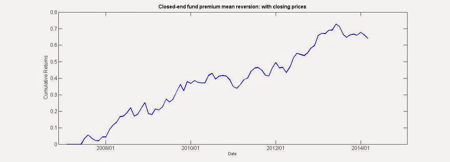
Patro et al published a paper on trading the mean reversion of closed-end funds’ (CEF) premium. Based on rational analysis, the market value of a CEF should be the same as the net asset value (NAV) of its holdings. So the strategy to exploit any differences is both reasonable and simple: rank all the CEF's by their % difference ("premium") between market value and NAV, and short the quintile with the highest premium and buy the quintile with the lowest (maybe negative) premium. Hold them for a month, and repeat. (You can try this on a daily basis too, since Bloomberg provides daily NAV data.) The Sharpe ratio of this strategy from 1998-2011 is 1.5. Transaction costs are ignored, but shouldn't be significant for a monthly rebalance strategy.

The authors are irreproachable for their use of high quality price data provided by CRSP and monthly fund NAV data from Bloomberg for their backtest. So I was quite confident that I can reproduce their results with the same data from CRSP, and with historical NAV data from Compustat instead. Indeed, here is the cumulative returns chart from my own backtest (click to enlarge):

However, I also know that there is one detail that many traders and academic researchers neglect when they backtest daily strategies for stocks, ETFs, or CEFs. They often use the "consolidated" closing price as the execution price, instead of the "official" (also called "auction" or "primary") closing price. To understand the difference, one has to remember that the US stock market is a network of over 60 "market centers" (see the teaching notes of Prof. Joel Hasbrouck for an excellent review of the US stock market structure). The exact price at which one's order will be executed is highly dependent on the exact market center to which it has been routed. A natural way to execute this CEF strategy is to send a market-on-close (MOC) or limit-on-close (LOC) order near the close, since this is the way we can participate in the closing auction and avoid paying the bid-ask spread. Such orders will be routed to the primary exchange for each stock, ETF, or CEF, and the price it is filled at will be the official/auction/primary price at that exchange. On the other hand, the price that most free data service (such as Yahoo Finance) provides is the consolidated price, which is merely that of the last transaction received by the Securities Information Processor (SIP) from any one of these market centers on or before 4pm ET. There is no reason to believe that one's order will be routed to that particular market center and was executed at that price at all. Unfortunately, the CEF strategy was tested on this consolidated price. So I decide to backtest it again with the official closing price.

Where can we find historical official closing price? Bloomberg provides that, but it is an expensive subscription. CRSP data has conveniently included the last bid and ask that can be used to compute the mid price at 4pm which is a good estimate of the official closing price. This mid price is what I used for a revised backtest. But the CRSP data also doesn't come cheap - I only used it because my academic affiliation allowed me free access. There is, however, an unexpected source that does provide the official closing price at a reasonable rate: QuantGo.com will rent us tick data that has a Cross flag for the closing auction trade. How ironic: the cheapest way to properly backtest a strategy that trades only once a month requires tick data time-stamped at 1 millisecond, with special tags for each trade!

So what is the cumulative returns using the mid price for our backtest?

Opening Gap Reversion

Readers of my book will be familiar with this strategy (Example 4.1): start with the SPX universe, buy the 10 stocks that gapped down most at the open, and short the 10 that gapped up most. Liquidate everything at the close. We can apply various technical or fundamental filters to make this strategy more robust, but the essential driver of the returns is mean-reversion of the overnight gap (i.e. reversion of the return from the previous close to today's open).

We have backtested this strategy using the closing mid price as I recommended above, and including a further 5 bps transaction cost each for the entry and exit trade. The backtest looked wonderful, so we traded it live. Here is the comparison of the backtest vs live cumulative P&L:

Yes, it is still mildly profitable, but nowhere near the profitability of the backtest, or more precisely, walk-forward test. What went wrong? Two things:

Just like the closing price, we should have used the official/auction/primary open price. Unfortunately CRSP does not provide the opening bid-ask, so we couldn't have estimated the open price from the mid price. QuantGo, though, does provide a Cross flag for the opening auction trade as well.
To generate the limit on open (LOO) or market on open (MOO) orders suitable for executing this strategy, we need to submit the order using the pre-market quotes before 9:28am ET, based on Nasdaq's rules.

Once again, a strategy that is seemingly low frequency, with just an entry at the open and an exit at the close, actually requires TAQ (ticks and quotes) data to backtest properly.

Futures Momentum

Lest you think that this requirement for TAQ data for backtesting only applies to mean reversion strategies, we can consider the following futures momentum strategy that can be applied to the gasoline (RB), gold (GC), or various other contracts trading on the NYMEX.

At the end of a trading session (defined as the previous day's open outcry close to today's open outcry close), rank all the trades or quotes in that session. We buy a contract in the next session if the last price is above the 95th percentile, sell it if it drops below the 60th (this serves as a stop loss). Similarly, we short a contract if the last price is below the 5th percentile, and buy cover if it goes above the 40th.

Despite being an intraday strategy, it typically trades only 1 roundtrip a day - a low frequency strategy. We backtested it two ways: with 1-min trade bars (prices are from back-adjusted continuous contracts provided by eSignal), and with best bid-offer (BBO) quotes with 1 ms time stamps (from QuantGo's actual contract prices, not backadjusted).

For all the contracts that we have tested, the 1-ms data produced much worse returns than the 1-min data. The reason is interesting: 1-ms data shows that the strategy exhibits high frequency flip-flops. These are sudden changes in the order book (in particular, BBO quotes) that quickly revert. Some observers have called these flip-flops "mini flash crashes", and they happen as frequently in the futures as in the stock market, and occasionally in the spot Forex market as well. Some people have blamed it on high frequency traders. But I think flip-flop describe the situation better than flash crash, since flash crash implies the sudden disappearance of quotes or liquidity from the order book, while in a flip-flopping situation, new quotes/liquidity above the BBO can suddenly appear and disappear in a few milliseconds, simultaneous with the disappearance and re-appearance of quotes on the opposite side of the order book. Since ours is a momentum strategy, such reversals of course create losses. These losses are very real, and we experienced it in live trading. But these losses are also undetectable if we backtest using 1-min bar data.

Some readers may object: if the 1-min bar backtest shows good profits, why not just trade this live with 1-min bar data and preserve its profit? Let's consider why this doesn't actually allow us to avoid using TAQ data. Note that we were able to avoid the flip-flops using 1-min data only because we were lucky in our backtest - it wasn't because we had some trading rule that prevented our entering or exiting a position when the flip-flops occurred. How then are we to ensure that our luck will continue with live market data? At the very least, we have to test this strategy with many sets of 1-min bar data, and choose the set that shows the worst returns as part of our stress testing. For example, one set may be [9:00:00, 9:01:00, 9:02:00, ...,] and the second set may be [9:00:00.001, 9:01:00.001, 9:02:00.001, ...], etc. This backtest, however, still requires TAQ data, since no historical data vendor I know of provides such multiple sets of time-shifted bars!

As I mentioned above, these flip-flops are omnipresent in the stock market as well. This shouldn't be surprising considering that 50% of the stock transaction volume is due to high frequency trading. It is particularly damaging when we are trading spreads, such as the ETF pair EWA vs EWC. A small change in the BBO of a leg may represent a big percentage change in the spread, which itself may be just a few ticks wide. So such flip-flops can frequently trigger orders which are filled at much worse prices than expected.

Conclusion

The three example strategies above illustrate that even when a strategy trades at low frequency, maybe as low as once a month, we often still require high frequency TAQ data to backtest it properly, or even economically. If the strategy trades intraday, even if just once a day, then this requirement becomes all the more important due to the flip-flopping of the order book in the millisecond time frame.

===

My Upcoming Talks and Workshops

5/13-14: "Mean Reversion Strategies", "AI techniques in Trading" and "Portfolio Optimization" at Q-Trade Bootcamp 2015, Milan, Italy.

5/18-22: "Statistical Arbitrage", 'Quantitative Momentum", and "Millisecond Frequency Trading", London, UK.

6/17-19: "Mean Reversion Strategies" live online workshop.

===

Managed Account Program Update

Our FX Managed Account program has a net return of +4.29% in March (YTD: +12.7%).

===

Follow me on Twitter: @chanep

Most time series techniques such as the ADF test for stationarity, Johansen test for cointegration, or ARIMA model for returns prediction, assume that our data points are collected at regular intervals. In traders' parlance, it assumes bar data with fixed bar length. It is easy to see that this mundane requirement immediately presents a problem even if we were just to analyze daily bars: how are we do deal with weekends and holidays?

You can see that the statistics of return bars over weekdays can differ significantly from those over weekends and holidays. Here is a table of comparison for SPY daily returns from 2005/05/04-2015/04/09:

SPY daily returns	Number of bars	Mean Returns (bps)	Mean Absolute Returns (bps)	Kurtosis (3 is “normal”)
Weekdays only	1,958	3.9	80.9	13.0
Weekends/holidays only	542	0.3	82.9	23.7

Though the absolute magnitude of the returns over a weekday is similar to that over a weekend, the mean returns are much more positive on the weekdays. Note also that the kurtosis of returns is almost doubled on the weekends. (Much higher tail risks on weekends with much less expected returns: why would anyone hold a position over weekends?) So if we run any sort of time series analysis on daily data, we are force-fitting a model on data with heterogeneous statistics that won't work well.

The problem is, of course, much worse if we attempt time series analysis on intraday bars. Not only are we faced with the weekend gap, in the case of stocks or ETFs we are faced with the overnight gap as well. Here is a table of comparison for AUDCAD 15-min returns vs weekend returns from 2009/01/01-2015/06/16:

AUDCAD 15-min returns	Number of bars	Mean Returns (bps)	Mean Absolute Returns (bps)	Kurtosis (3 is “normal”)
Weekdays only	158,640	0.01	4.5	18.8
Weekends/holidays only	343	-2.06	15.3	4.6

In this case, every important statistic is different (and it is noteworthy that kurtosis is actually lower on the weekends here, illustrating the mean-reverting character of this time series.)

So how should we predict intraday returns with data that has weekend gaps? (The same solution should apply to overnight gaps for stocks, and so omitted in the following discussion.) Let's consider several proposals:

1) Just delete the weekend returns, or set them as NaN in Matlab, or missing values NA in R.

This won't work because the first few bars of a week isn't properly predicted by the last few bars of the previous week. We shouldn't use any linear model built with daily or intraday data to predict the returns of the first few bars of a week, whether or not that model contains data with weekend gaps. As for how many bars constitute the "first few bars", it depends on the lookback of the model. (Notice I emphasize linear model here because some nonlinear models can deal with large jumps during the weekends appropriately.)

2) Just pretend the weekend returns are no different from the daily or intraday returns when building/training the time series model, but do not use the model for predicting weekend returns. I.e. do not hold positions over the weekends.

This has been the default, and perhaps simplest (naive?) way of handling this issue for many traders, and it isn't too bad. The predictions for the first few bars in a week will again be suspect, as in 1), so one may want to refrain from trading then. The model built this way isn't the best possible one, but then we don't have to be purists.

3) Use only the most recent period without a gap to train the model. So for an intraday FX model, we would be using the bars in the previous week, sans the weekends, to train the model. Do not use the model for predicting weekend returns nor the first few bars of a week.

This sounds fine, except that there is usually not enough data in just a week to build a robust model, and the resulting model typically suffers from severe data snooping bias.

You might think that it should be possible to concatenate data from multiple gapless periods to form a larger training set. This "concatenation" does not mean just piecing together multiple weeks' time series into one long time series - that would be equivalent to 2) and wrong. Concatenation just means that we maximize the total log likelihood of a model over multiple independent time series, which in theory can be done without much fuss since log likelihood (i.e. log probability) of independent data are additive. But in practice, most pre-packaged time series model programs do not have this facility. (Do add a comment if anyone knows of such a package in Matlab, R, or Python!) Instead of modifying the guts of a likelihood-maximization routine of a time series fitting package, we will examine a short cut in the next proposal.

4) Rather than using a pre-packaged time series model with maximum likelihood estimation, just use an equivalent multiple linear regression (LR) model. Then just fit the training data with this LR model with all the data in the training set except the weekend bars, and use it for predicting all future bars except the weekend bars and the first few bars of a week.

This conversion of a time series model into a LR model is fairly easy for an autoregressive model AR(p), but may not be possible for an autoregressive moving average model ARMA(p, q). This is because the latter involves a moving average of the residuals, creating a dependency which I don't know how to incorporate into a LR. But I have found that AR(p) model, due to its simplicity, often works better out-of-sample than ARMA models anyway. It is of course, very easy to just omit certain data points from a LR fit, as each data point is presumed independent.

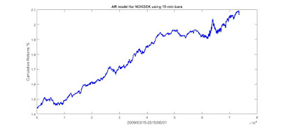
Here is a plot of the out-of-sample cumulative returns of one such AR model built for predicting 15-minute returns of NOKSEK, assuming midpoint executions and no transaction costs (click to enlarge.)

Whether or not one decides to use this or the other techniques for handling data gaps, it is always a good idea to pay some attention to whether a model will work over these special bars.

===

My Upcoming Workshop

July 29-30: Artificial Intelligence Techniques for Traders.

This is a new online workshop focusing on the practical use of AI techniques for identifying predictive indicators for asset returns.

===

Managed Accounts Update

Our FX Managed Account program is 6.02% in June (YTD: 31.33%).

===

Industry Update

I previously reported on a fundamental stock model proposed by Lyle and Wang using a linear combination of just two firm fundamentals ― book-to-market ratio and return on equity. Professor Lyle has posted a new version of this model.

Charles-Albert Lehalle, Jean-Philippe Bouchaud, and Paul Besson reported that "intraday price is more aligned to signed limit orders (cumulative order replenishment) rather than signed market orders (cumulative order imbalance), even if order imbalance is able to forecast short term price movements." Hat tip: Mattia Manzoni. (I don't have a link to the original paper: please ask Mattia for that!)

A new investment competition to help you raise capital is available at hedgefol.io.

Enjoy an Outdoor Summer Party with fellow quants benefiting the New York Firefighters Burn Center Foundation on Tuesday, July 14th with great food and cool drinks on a terrace overlooking Manhattan. Please RSVP to join quant fund managers, systematic traders, algorithmic traders, quants and high frequency sharks for a great evening. This is a complimentary event (donations are welcomed).

===

Follow me on Twitter: @chanep

I have been a big fan of options trader and author Euan Sinclair for a long time. I have cited his highly readable and influential book Option Trading in my own work, and it is always within easy reach from my desk. His more recent book Volatility Trading is another must-read. I ran into him at the Chicago Trading Show a few months ago where he was a panelist on volatility trading, and he graciously agreed to be interviewed by me.

What is your educational background, and how did you start your trading career?

I got a Ph.D. in theoretical physics, studying the transition from quantum to classical mechanics. I always had intended to become a professor but the idea became less appealing once I saw what they did all day. At this time Nick Leeson was making news by blowing up Barings Bank and I thought I could do that. I mean trade derivatives not blowing up a bank (although I could probably manage that as well).

Do you recommend a new graduate with a similar educational background as yours to pursue finance or trading as a career today?

I don't think I would for a few reasons.

The world of derivatives and trading in general is now so much more visible than it was and there are now far better ways to prepare. When I started, physics Ph.D.s were hired only because they were smart and numerate and could pick things up on their own. My first trading firm had no training program. You just had to figure stuff out on your own. Now there are many good MFE courses or you could do a financial economics Ph.D.

Further, it would very much depend on exactly what kind of physics had been studied. I did a lot of classical mechanics which is really geometry. This kind of "pure" theory isn't nearly as useful as a background heavy with stats or simulation.

I think I could still make the transition, but it is no longer close to the ideal background.

You have been a well-known options trader with a long track record: what do you think is the biggest obstacle to success for a retail options trader?

Trading costs. Most option trading ideas are still built on the Black-Scholes-Merton framework and the idea of dynamic hedging (albeit heavily modified). Most pro firms have stat arb like execution methods to reduce the effective bid-ask they pay in the underlying. They also pay practically no ticket charges and probably get rebates. Even then, their average profit per option trade is very small and has been steadily decreasing.

Further, a lot of positional option trading relies on a large universe of possible trades to consider. This means a trader needs good scanning software to find trades, and a decent risk system because she will tend to have hundreds of positions on at one time. This is all expensive as well.

Retail traders can't play this game at all. They have to look for situations that require little or no rebalancing and that can be limited to a much smaller universe. I would recommend the VIX complex or equity earnings events.

As an options trader, do you tend to short or long volatility?

I am short about 95% of the time, but about 35% of my profits come from the long trades.

Do you find it possible to fully automate options trading in the same way as that stocks, futures, and FX trading have been automated?

I see no reason why not.

You have recently started a new website called FactorWave.com. Can you tell us about it? What prompted the transition of your focus from options to stocks?

FactorWave is a set of stock and portfolio tools that do analysis in terms of factors such as value, size, quality and momentum. There is a lot of research by both academics and investors that shows that these (and other) factors can give market beating returns and lower volatility.

I've been interested in stocks for a long time. Most of my option experience has been with stock options and some of my best research was on how these factors affected volatility trading returns.Also, equity markets are a great place to build wealth over the long term. They are a far more suitable vehicle for retirement planning than options!

I actually think the distinction between trading and investing is fairly meaningless. The only difference seems to be the time scale and this is very dependent on the person involved as well, with long-term meaning anything form months to inter-generational. All I've ever done as a trader is to look for meaningful edges and I found a lot of these in options. But I've never found anything as persistent as the stock factors. There is over a hundred years of statistical evidence, studies in many countries and economic and behavioral reasons for their existence. They present some of the best edges I have ever found. That should be appealing to any trader or investor.

Thank you! These are really valuable insights.

====

My Upcoming Workshop

October 28-29: Quantitative Momentum Strategies.

Momentum strategies have performed superbly in the recent market turmoil, since they are long volatility. This course will cover momentum strategies on a variety of asset classes and with a range of trading horizons.

====

QTS Partners, L.P. has a net return of 1.25% in August (YTD: 10.44%).

====

Reader Burak B. has converted some of the Matlab codes from my book Algorithmic Trading into Python codes and made them open-source: https://github.com/burakbayramli/quant_at.

====

Follow me on Twitter: @chanep

By Lukasz Wojtow

Mechanical traders never stop researching for the next market edge. Not only to get better results but also to have more than one system. The best trading results can be achieved with multiple non-correlated systems traded simultaneously. Unfortunately, most traders use similar market inefficiency: some traders specialize in trend following, some in mean reversion and so on. That's because learning to exploit one kind of edge is hard enough, mastering all of them – impossible. It would be beneficial to have a software that creates many non-related systems.

Recently I released Genotick - an open source software that can create and manage a group of trading systems. At the Genotick's core lies an epiphany: if it's possible to create any software with just a handful of assembler instructions, it should be possible to create any trading systems with a handful of similarly simple instructions. These simple and meaningless-on-its-own instructions become extremely powerful when combined together. Right instructions in the right order can create any type of mechanical system: trend following, mean reverting or even based on fundamental data.

The driving engine behind Genotick's power is a genetic algorithm. Current implementation is quite basic, but with some extra quirks. For example, if any of the systems is really bad – it stays in the population but its predictions are reversed. Another trick is used to help recognize biased trading systems: a system can be removed if it doesn't give mirrored prediction on mirrored data. So for example, position on GBP/USD must be opposite to the one on USD/GBP. Genotick also supports optional elitism (where the best systems always stay in the population, while others are retired due to old age), protection for new systems (to avoid removing systems that didn't yet have a chance to prove themselves) and inheriting initial system's weight from parents. These options give users plenty of room for experimentation.

When Genotick is run for the first time - there are no systems. They are created at the start using randomly chosen instructions. Then, a genetic algorithm takes over: each system is executed to check its prediction on historical data. Systems that predicted correctly gain weight for future predictions, systems that predicted incorrectly – lose weight. Gradually, day after day, population of systems grows. Bad systems are removed and good systems breed. Prediction for each day is calculated by adding predictions of all systems available at the time. Genotick doesn't iterate over the same historical data more than once – training process looks exactly as if it was executed in real life: one day at a time. In fact, there is no separate “training” phase, program learns a little bit as each day passes by.

Interestingly, Genotick doesn't check for rationale behind created systems. As each system is created out of random instructions, it's possible (and actually very likely) that some systems use ridiculous logic. For example, it's possible that a system will give a “Buy” signal if Volume was positive 42 days ago. Another system may want to go short each time the third digit in yesterday's High is the same as second digit in today's Open. Of course, such systems would never survive in real world and also they wouldn't survive for long in Genotick's population. Because each system's initial weight is zero, they never gain any significant weight and therefore don't spoil cumulative prediction given by the program. It may seem a little silly to allow such systems in the first place, but it enables Genotick to test algorithms that are free from traders' believes, misguided opinions and personal limitations. The sad fact is, the market doesn't care about what system you use and how much sweat and tears you put into it. Market is going to do what it wants to do – no questions asked, not taking prisoners. Market doesn't even care if you use any sort of intelligence, artificial or not. And so, the only rationale behind every trading system should be very simple: “Does it work?”. Nothing more, nothing less. This is the only metric Genotick uses to gauge systems.

Each program's run will be a little bit different. Equity chart below shows one possible performance. Years shown are 2007 until 2015 with actual training starting in 2000. There is nothing special about year 2007, remember – Genotick learns as it goes along. However, I felt it's important to look how it performed during financial crisis. Markets traded were:

USD/CHF, USD/JPY, 10 Year US Bond Yield, SPX, EUR/USD, GBP/USD and Gold.

(In some cases, I tested the system on a market index such as SPX instead of an instrument that tracks the index such as SPY, but the difference should be minor.) All markets were mirrored to allow removing biased systems. Some vital numbers:

CAGR: 9.88%
Maxim drawdown: -21.6%
Longest drawdown: 287 trading days
Profitable days: 53.3 %
CALMAR ratio: 0.644
Sharpe ratio: 1.06
Mean annual gain: 24.1%
Losing year: 2013 (-12%)

(Click the cumulative returns in % chart below to enlarge.)

Cumulative Returns (%) since 2007

These numbers represent only “directional edge” offered by the software. There were no stop-losses, no leverage and no position sizing, which could greatly improve real life results. The performance assumes that at the end of each day, the positions are rebalanced so that each instrument starts with equal dollar value. (I.e. this is a constant rebalanced portfolio.)

Artificial Intelligence is a hot topic. Self driving cars that drive better than an average human and chess algorithms that beat an average player are facts. The difference is that using AI for trading is perfectly legal and opponents may never know. Unlike chess and driving, there is a lot of randomness in financial markets and it may take us longer to notice when AI starts winning. Best hedge funds can be still run by humans but if any trading method is really superior, AI will figure it out as well.

At the moment Genotick is more of a proof-of-concept rather than production-ready.

It is very limited in usability, it doesn't forgive mistakes and it's best to ask before using it for real trading. You will need Java 7 to run it. It's tested on both Linux and Windows 10. Example historical data is included. Any questions or comments are welcomed.

Genotick website: http://genotick.com

Source code: http://github.com/alphatica/genotick

Forum: https://groups.google.com/forum/#!forum/genotick

For a general reference on genetic algorithms, see "How to Solve It: Modern Heuristics".

===

My Upcoming Workshop

October 28-29: Quantitative Momentum Strategies.

====

Follow me on Twitter: @chanep

Predicting volatility is a very old topic. Every finance student has been taught to use the GARCH model for that. But like most things we learned in school, we don't necessarily expect them to be useful in practice, or to work well out-of-sample. (When was the last time you need to use calculus in your job?) But out of curiosity, I did a quick investigation of its power on predicting the volatility of SPY daily close-to-close returns. I estimated the parameters of a GARCH model on training data from December 21, 2005 to December 5, 2011 using Matlab's Econometric toolbox, and tested how often the sign of the predicted 1-day change in volatility agree with reality on the test set from December 6, 2011 to November 25, 2015. (One-day change in realized volatility is defined as the change in the absolute value of the 1-day return.) A pleasant surprise: the agreement is 58% of the days.

If this were the accuracy for predicting the sign of the SPY return itself, we should prepare to retire in luxury. Volatility is easier to predict than signed returns, as every finance student has also been taught. But what good is a good volatility prediction? Would that be useful to options traders, who can trade implied volatilities instead of directional returns? The answer is yes, realized volatility prediction is useful for implied volatility prediction, but not in the way you would expect.

If GARCH tells us that the realized volatility will increase tomorrow, most of us would instinctively go out and buy ourselves some options (i.e. implied volatility). In the case of SPY, we would probably go buy some VXX. But that would be a terrible mistake. Remember that the volatility we predicted is an unsigned return: a prediction of increased volatility may mean a very bullish day tomorrow. A high positive return in SPY is usually accompanied by a steep drop in VXX. In other words, an increase in realized volatility is usually accompanied by a decrease in implied volatility in this case. But what is really strange is that this anti-correlation between change in realized volatility and change in implied volatility also holds when the return is negative (57% of the days with negative returns). A very negative return in SPY is indeed usually accompanied by an increase in implied volatility or VXX, inducing positive correlation. But on average, an increase in realized volatility due to negative returns is still accompanied by a decrease in implied volatility.

The upshot of all these is that if you predict the volatility of SPY will increase tomorrow, you should short VXX instead.

====

Industry Update

Quantiacs.com just launched a trading system competition with guaranteed investments of $2.25M for the best three trading systems. (Quantiacs helps Quants get investments for their trading algorithms and helps investors find the right trading system.)
A new book called "Momo Traders - Tips, Tricks, and Strategies from Ten Top Traders" features extensive interviews with ten top day and swing traders who find stocks that move and capitalize on that momentum.
Another new book called "Algorithmic and High-Frequency Trading" by 3 mathematical finance professors describes the sophisticated mathematical tools that are being applied to high frequency trading and optimal execution. Yes, calculus is required here.

My Upcoming Workshop

January 27-28: Algorithmic Options Strategies

This is a new online course that is different from most other options workshops offered elsewhere. It will cover how one can backtest intraday option strategies and portfolio option strategies.

March 7-11: Statistical Arbitrage, Quantitative Momentum, and Artificial Intelligence for Traders.

These courses are highly intensive training sessions held in London for a full week. I typically need to walk for an hour along the Thames to rejuvenate after each day's class.

The AI course is new, and to my amazement, some of the improved techniques actually work.

My Upcoming Talk

I will be speaking at QuantCon 2016 on April 9 in New York. The topic will be "The Peculiarities of Volatility". I pointed out one peculiarity above, but there are others.

====

QTS Partners, L.P. has a net return of +1.56% in October (YTD: +11.50%). Details available to Qualified Eligible Persons as defined in CFTC Rule 4.7.

====

Follow me on Twitter: @chanep

Everybody know that volatility depends on the measurement frequency: the standard deviation of 5-minute returns is different from that of daily returns. To be precise, if z is the log price, then volatility, sampled at intervals of τ, is

volatility(τ)=√(Var(z(t)-z(t-τ)))

where Var means taking the variance over many sample times. If the prices really follow a geometric random walk, then Var(τ)≡Var((z(t)-z(t-τ)) ∝ τ, and the volatility simply scales with the square root of the sampling interval. This is why if we measure daily returns, we need to multiply the daily volatility by √252 to obtain the annualized volatility.

Traders also know that prices do not really follow a geometric random walk. If prices are mean reverting, we will find that they do not wander away from their initial value as fast as a random walk. If prices are trending, they wander away faster. In general, we can write

Var(τ) ∝ τ^(2H)

where H is called the "Hurst exponent", and it is equal to 0.5 for a true geometric random walk, but will be less than 0.5 for mean reverting prices, and greater than 0.5 for trending prices.

If we annualize the volatility of a mean-reverting price series, it will end up having a lower annualized volatility than that of a geometric random walk, even if both have exactly the same volatility measured at, say, 5-min bars. The opposite is true for a trending price series. For example, if we try this on AUDCAD, an obviously mean-reverting time series, we will get H=0.43.

All of the above are well-known to many traders, and are in fact discussed in my book. But what is more interesting is that the Hurst exponent itself can change at some time scale, and this change sometimes signals a shift from a mean reversion to a momentum regime, or vice versa. To see this, let's plot volatility (or more conveniently, variance) as a function of τ. This is often called the term structure of (realized) volatility.

Start with the familiar SPY. we can compute the intraday returns using midprices from 1 minutes to 2^10 minutes (~17 hrs), and plot the log(Var(τ)) against log(τ). The fit, shown below, is excellent. (Click figure to enlarge). The slope, divided by 2, is the Hurst exponent, which turns out to be 0.494±0.003, which is very slightly mean-reverting.

But if we do the same for daily returns of SPY, for intervals of 1 day up to 2^8 (=256) days, we find that H is now 0.469±0.007, which is significantly mean reverting.

Conclusion: mean reversion strategies on SPY should work better interday than intraday.

We can do the same analysis for USO (the WTI crude oil futures ETF). The intraday H is 0.515±0.001, indicating significant trending behavior. The daily H is 0.56±0.02, even more significantly trending. So momentum strategies should work for crude oil futures at any reasonable time scales.

Let's turn now to GLD, the gold ETF. Intraday H=0.505±0.002, which is slightly trending. But daily H=0.469±0.007: significantly mean reverting! Momentum strategies on gold may work intraday, but mean reversion strategies certainly work better over multiple days. Where does the transition occur? We can examine the term structure closely:

We can see that at around 16-32 days, the volatilities depart from straight line extrapolated from intraday frequencies. That's where we should switch from momentum to mean reversion strategies.

One side note of interest: when we compute the variance of returns over periods that straddle two trading days and plot them as function of log(τ), should τ include the hours when the market was closed? It turns out that the answer is yes, but not completely. In order to produce the chart above where the daily variances initially fall on the same straight line as the intraday variances, we have to count 1 trading day as equivalent to 10 trading hours. Not 6.5 (for the US equities/ETF markets), and not 24. The precise number of equivalent trading hours, of course, varies across different instruments.

===

Industry Update

Nick over at mintegration.eu discusses the new intraday databases at Quandl and Kerf.
Factorwave.com (Euan Sinclair's creation) started a new forum: slack.factorwave.com. It has some very active and in-depth discussions of many trading and investing topics.
Prof. Matthew Lyle at Kellogg School of Management has a new paper out that relates fundamentals to variance risk premiums: http://papers.ssrn.com/sol3/papers.cfm?abstract_id=2696183.

Upcoming Workshops

April 20-21: Mean Reversion Strategies.

There are a lot more to mean reversion strategies than just pairs trading. Find out how to thrive in the current low volatility environment favorable to this type of strategies.

Everybody loves trading or investing in ETPs. ETP is the acronym for exchange-traded products, which include both exchange-traded funds (ETF) and exchange-traded notes (ETN). They seem simple, transparent, easy to understand. But there are a few subtleties that you may not know about.

1) The most popular ETN is VXX, the volatility index ETF. Unlike ETF, ETN is actually an unsecured bond issued by the issuer. This means that the price of the ETN may not just depend on the underlying assets or index. It could potentially depend on the credit-worthiness of the issuer. Now VXX is issued by Barclays. You may think that Barclays is a big bank, Too Big To Fail, and you may be right. Nevertheless, nobody promises that its credit rating will never be downgraded. Trading the VX future, however, doesn't have that problem.

2) The ETP issuer, together with the "Authorized Participants" (the market makers who can ask the issuer to issue more ETP shares or to redeem such shares for the underlying assets or cash), are supposed to keep the total market value of the ETP shares closely tracking the NAV of the underlying assets. However, there was one notable instance when the issuer deliberately not do so, resulting in big losses for some investors.

That was when the issuer of TVIX, the leveraged ETN that tracks 2x the daily returns of VXX, stopped all creation of new TVIX shares temporarily on February 22, 2012 (see sixfigureinvesting.com/2015/10/how-does-tvix-work/). That issuer is Credit Suisse, who might have found that the transaction costs of rebalancing this highly volatile ETN were becoming too high. Because of this stoppage, TVIX turned into a closed-end fund (temporarily), and its NAV diverged significantly from its market value. TVIX was trading at a premium of 90% relative to the underlying index. In other words, investors who bought TVIX in the stock market by the end of March were paying 90% more than they would have if they were able to buy the VIX index instead. Right after that, Credit Suisse announced they would resume the creation of TVIX shares. The TVIX market price immediately plummeted to its NAV per share, causing huge losses for those investors who bought just before the resumption.

3) You may be familiar with the fact that a β-levered ETF is supposed to track only β times the daily returns of the underlying index, not its long-term return. But you may be less familiar with the fact that it is also not supposed to track β times the intraday return of that index (although at most times it actually does, thanks to the many arbitrageurs.)

Case in point: during the May 2010 Flash Crash, many inverse levered ETFs experienced a decrease in price as the market was crashing downwards. As inverse ETFs, many investors thought they are supposed to rise in price and act as hedge against market declines. For example, this comment letter to the SEC pointed out that DOG, the inverse ETF that tracks -1x Dow 30 index, went down more than 60% from its value at the beginning (2:40 pm ET) of the Flash Crash. This is because various market makers including the Authorized Participants for DOG weren't making markets at that time. But an equally important point to note is that at the end of the trading day, DOG did return 3.2%, almost exactly -1x the return of DIA (the ETF that tracks the Dow 30). So it functioned as advertised. Lesson learned: We aren't supposed to use inverse ETFs for intraday nor long term hedging!

4) The NAV (not NAV per share) of an ETF does not have to change in the same % as the underlying asset's unit market value. For example, that same comment letter I quoted above wrote that GLD, the gold ETF, declined in price by 24% from March 1 to December 31, 2013, tracking the same 24% drop in spot gold price. However, its NAV dropped 52%. Why? The Authorized Participants redeemed many GLD shares, causing the shares outstanding of GLD to decrease from 416 million to 266 million. Is that a problem? Not at all. An investor in that ETF only cares that she experienced the same return as spot gold, and not how much assets the ETF held. The author of that comment letter strangely wrote that "Investors wishing to participate in the gold market would not buy the GLD if they knew that a price decline in gold could result in twice as much underlying asset decline for the GLD." That, I believe, is nonsense.

For further reading on ETP, see www.ici.org/pdf/per20-05.pdf and www.ici.org/pdf/ppr_15_aps_etfs.pdf.

===

Industry Update

Alex Boykov co-developed the WFAToolbox– Walk-Forward Analysis Toolbox for MATLAB, which automates the process of using a moving window to optimize parameters and entering trades only in the out-of-sample period. He also compiled a standalone application from MATLAB that allows any user (having MATLAB or not) to upload quotes in csv format from Google Finance for further import to other programs and for working in Excel. You can download it here: wfatoolbox.com/epchan.

Upcoming Workshop

July 16 and 23, Saturdays: Artificial Intelligence Techniques for Traders.

AI/machine learning techniques are most useful when someone gives us newfangled technical or fundamental indicators, and we haven't yet developed the intuition of how to use them. AI techniques can suggest ways to incorporate them into your trading strategy, and quicken your understanding of these indicators. Of course, sometimes these techniques can also suggest unexpected strategies in familiar markets.

My course covers the basic AI techniques useful to a trader, with emphasis on the many ways to avoid overfitting.

I wrote in a previous article about why we should backtest even end-of-day (daily) strategies with intraday quote data. Otherwise, the performance of such strategies can be inflated. Here is another brilliant example that I came across recently.

Consider the oil futures ETF USO and its evil twin, the inverse oil futures ETF DNO*. In theory, if USO has a daily return of x%, DNO will have a daily return of -x%. In practice, if we plot the daily returns of DNO against that of USO from 2010/9/27-2016/9/9, using the usual consolidated end-of-day data that you can find on Yahoo! Finance or any other vendor,

we see that though the slope is indeed -1 (to within a standard error of 0.004), there are many days with significant deviation from the straight line. The trader in us will immediately think "arbitrage opportunities!"

Indeed, if we backtest a simple mean reversion strategy on this pair - just buy equal dollar amount of USO and DNO when the sum of their daily returns is less than 40 bps at the market close, hold one day, and vice versa - we will find a strategy with a decent Sharpe ratio of 1 even after deducting 5 bps per side as transaction costs. Here is the equity curve:

Looks reasonable, doesn't it? However, if we backtest this strategy again with BBO data at the market close, taking care to subtract half the bid-ask spread as transaction cost, we find this equity curve:

We can see that the problem is not only that we lose money on practically every trade, but that there was seldom any trade triggered. When the daily EOD data suggests a trade should be triggered, the 1-min bar BBO data tells us that in fact there was no deviation from the mean.

(By the way, the returns above were calculated before we even deduct the borrow costs of occasionally shorting these ETFs. The "rebate rate" for USO is about 1% per annum on Interactive Brokers, but a steep 5.6% for DNO.)

In case you think this problem is peculiar to USO vs DNO, you can try TBT vs UBT as well.

Incidentally, we have just verified a golden rule of financial markets: apparent deviation from efficient market is allowed when no one can profitably trade on the arbitrage opportunity.

===
*Note: according to www.etf.com, "The issuer [of DNO] has temporarily suspended creations for this fund as of Mar 22, 2016 pending the filing of new paperwork with the SEC. This action could create unusual or excessive premiums— an increase of the market price of the fund relative to its fair value. Redemptions are not affected. Trade with care; check iNAV vs. price." For an explanation of "creation" of ETF units, see my article "Things You Don't Want to Know about ETFs and ETNs".

===

Industry Update

Quantiacs.com just recently registered as a CTA and operates a marketplace for trading algorithms that anyone can contribute. They also published an educational blog post for Python and Matlab backtesters: https://quantiacs.com/Blog/Intro-to-Algorithmic-Trading-with-Heikin-Ashi.aspx

I will be moderating a panel discussion on "How can funds leverage non-traditional data sources to drive investment returns?" at Quant World Canada in Toronto, November 10, 2016.

===

Upcoming Workshops

October 22 and 29, Saturdays, Quantitative Momentum Strategies online workshops.

Momentum strategies are for those who want to benefit from tail events. I will discuss the fundamental reasons for the existence of momentum in various markets, as well as specific momentum strategies that hold positions from hours to days.

A senior director at a major bank wrote me: "…thank you again for the Momentum Strategies training course this week. It was very beneficial. I found your explanations of the concepts very clear and the examples well developed. I like the rigorous approach that you take to strategy evaluation.”

Much has been written about the Post-Earnings Announcement Drift (PEAD) strategy (see, for example, my book), but less was written about pre-earnings announcement strategies. That changed recently with the publication of two papers. Just as with PEAD, these pre-announcement strategies do not make use of any actual earnings numbers or even estimates. They are based entirely on announcement dates (expected or actual) and perhaps recent price movement.

The first one, by So and Wang 2014, suggests various simple mean reversion strategies for US stocks that enter into positions at the market close just before an expected announcement. Here is my paraphrase of one such strategies:

1) Suppose t is the expected earnings announcement date for a stock in the Russell 3000 index.
2) Compute the pre-announcement return from day t-4 to t-2 (counting trading days only).
3) Subtract a market index return over the same lookback period from the pre-announcement return, and call this market-adjusted return PAR.
4) Pick the 18 stocks with the best PAR and short them (with equal dollars) at the market close of t-1, liquidate at market close of t+1. Pick the 18 stocks with the worst PAR, and do the opposite. Hedge any net exposure with a market-index ETF or future.

I backtested this strategy using Wall Street Horizon (WSH)'s expected earnings dates data, applying it to stocks in the Russell 3000 index, and hedging with IWV. I got a CAGR of 9.1% and a Sharpe ratio of 1 from 2011/08/03-2016/09/30. The equity curve is displayed below.

Note that WSH's data was used instead of Yahoo! Finance, Compustat, or even Thomson Reuters' I/B/E/S earnings data, because only WSH's data is "point-in-time". WSH captured the expected earnings announcement date on the day before the announcement, just as we would have if we were live trading. We did not use the actual announcement date as captured in most other data sources because we could not be sure if a company changed their expected announcement date on that same date. The actual announcement date can only be known with certainty after-the-fact, and therefore isn't point-in-time. If we were to run the same backtest using Yahoo! Finance's historical earnings data, the CAGR would have dropped to 6.8%, and the Sharpe ratio dropped to 0.8.

The notion that companies do change their expected announcement dates takes us to the second strategy, created by Ekaterina Kramarenko of Deltix's Quantitative Research Team. In her paper "An Automated Trading Strategy Using Earnings Date Movements from Wall Street Horizon", she describes the following strategy that explicitly makes use of such changes as a trading signal:

1) At the market close prior to the earnings announcement expected between the current close and the next day's open, compute deltaD which is the last change of the expected announcement date for the upcoming announcement, measured in calendar days. deltaD > 0 if the company moved the announcement date later, and deltaD < 0 if the company moved the announcement date earlier.
2) Also, at the same market close, compute deltaU which is the number of calendar days since the last change of the expected announcement date.
3) If deltaD < 0 and deltaU < 45, buy the stock at the market close and liquidate on next day's market open. If deltaD > 0 and deltaU >= 45, do the opposite.

The intuition behind this strategy is that if a company moves an expected announcement date earlier, especially if that happens close to the expected date, that is an indication of good news, and vice versa. Kramarenko found a CAGR of 14.95% and a Sharpe ratio of 2.08 by applying this strategy to SPX stocks from 2006/1/3 - 2015/9/2.

In order to reproduce this result, one needs to make sure that the capital allocation is based on the following formula: suppose the total buying power is M, and the number of trading signals at the market close is n, then the trading size per stock is M/5 if n <= 5, and is M/n if n > 5.

I backtested this strategy from 2011/8/3-2016/9/30 on a fixed SPX universe on 2011/7/5, and obtained CAGR=17.6% and Sharpe ratio of 0.6.

Backtesting this on Russell 3000 index universe of stocks yielded better results, with CAGR=17% and Sharpe ratio=1.9. Here, I adjust the trading size per stock to M/30 if n <=30, and to M/n if n > 30, given that the total number of stocks in Russell 3000 is about 6 times larger than that of SPX. The equity curve is displayed below:

Interestingly, a market neutral version of this strategy (using IWV to hedge any net exposure) does not improve the Sharpe ratio, but does significantly depressed the CAGR.

===

Acknowledgement: I thank Michael Raines at Wall Street Horizon for providing the historical point-in-time expected earning dates data for this research. Further, I thank Stuart Farr and Ekaterina Kramarenko at Deltix for providing me with a copy of their paper and explaining to me the nuances of their strategy.

===

My Upcoming Workshop

January 14 and 21: Algorithmic Options Strategies

This online course is different from most other options workshops offered elsewhere. It will cover backtesting intraday option strategies and portfolio option strategies.

One of the perennial problems in building trading models is the spareness of data and the attendant danger of overfitting. Fortunately, there are systematic methods of dealing with both ends of the problem. These methods are well-known in machine learning, though most traditional machine learning applications have a lot more data than we traders are used to. (E.g. Google used 10 million YouTube videos to train a deep learning network to recognize cats' faces.)

To create more training data out of thin air, we can resample (perhaps more vividly, oversample) our existing data. This is called bagging. Let's illustrate this using a fundamental factor model described in my new book. It uses 27 factor loadings such as P/E, P/B, Asset Turnover, etc. for each stock. (Note that I call cross-sectional factors, i.e. factors that depend on each stock, "factor loadings" instead of "factors" by convention.) These factor loadings are collected from the quarterly financial statements of SP 500 companies, and are available from Sharadar's Core US Fundamentals database (as well as more expensive sources like Compustat). The factor model is very simple: it is just a multiple linear regression model with the next quarter's return of a stock as the dependent (target) variable, and the 27 factor loadings as the independent (predictor) variables. Training consists of finding the regression coefficients of these 27 predictors. The trading strategy based on this predictive factor model is equally simple: if the predicted next-quarter-return is positive, buy the stock and hold for a quarter. Vice versa for shorts.

Note there is already a step taken in curing data sparseness: we do not try to build a separate model with a different set of regression coefficients for each stock. We constrain the model such that the same regression coefficients apply to all the stocks. Otherwise, the training data that we use from 200701-201112 will only have 1,260 rows, instead of 1,260 x 500 = 630,000 rows.

The result of this baseline trading model isn't bad: it has a CAGR of 14.7% and Sharpe ratio of 1.8 in the out-of-sample period 201201-201401. (Caution: this portfolio is not necessarily market or dollar neutral. Hence the return could be due to a long bias enjoying the bull market in the test period. Interested readers can certainly test a market-neutral version of this strategy hedged with SPY.) I plotted the equity curve below.

Next, we resample the data by randomly picking N (=630,000) data points with replacement to form a new training set (a "bag"), and we repeat this K (=100) times to form K bags. For each bag, we train a new regression model. At the end, we average over the predicted returns of these K models to serve as our official predicted returns. This results in marginal improvement of the CAGR to 15.1%, with no change in Sharpe ratio.

Now, we try to reduce the predictor set. We use a method called "random subspace". We randomly pick half of the original predictors to train a model, and repeat this K=100 times. Once again, we average over the predicted returns of all these models. Combined with bagging, this results in further marginal improvement of the CAGR to 15.1%, again with little change in Sharpe ratio.

The improvements from either method may not seem large so far, but at least it shows that the original model is robust with respect to randomization.

But there is another method in reducing the number of predictors. It is called stepwise regression. The idea is simple: we pick one predictor from the original set at a time, and add that to the model only if BIC (Bayesian Information Criterion) decreases. BIC is essentially the negative log likelihood of the training data based on the regression model, with a penalty term proportional to the number of predictors. That is, if two models have the same log likelihood, the one with the larger number of parameters will have a larger BIC and thus penalized. Once we reached minimum BIC, we then try to remove one predictor from the model at a time, until the BIC couldn't decrease any further. Applying this to our fundamental factor loadings, we achieve a quite significant improvement of the CAGR over the base model: 19.1% vs. 14.7%, with the same Sharpe ratio.

It is also satisfying that the stepwise regression model picked only two variables out of the original 27. Let that sink in for a moment: just two variables account for all of the predictive power of a quarterly financial report! As to which two variables these are - I will reveal that in my talk at QuantCon 2017 on April 29.

===

My Upcoming Workshops

March 11 and 18: Cryptocurrency Trading with Python

I will be moderating this online workshop for my friend Nick Kirk, who taught a similar course at CQF in London to wide acclaim.

May 13 and 20: Artificial Intelligence Techniques for Traders

I will discuss in details AI techniques such as those described above, with other examples and in-class exercises. As usual, nuances and pitfalls will be covered.

I have been troubled by the following paradox in the past few years. If a stock's log returns (i.e. change in log price per unit time) follow a Gaussian distribution, and if its net returns (i.e. percent change in price per unit time) have mean m and standard distribution s, then many finance students know that the mean log returns is m-s2 /2. That is, the compound growth rate of the stock is m-s2 /2. This can be derived by applying Ito's lemma to the log price process (see e.g. Hull), and is intuitively satisfying because it is saying that the expected compound growth rate is lowered by risk ("volatility"). OK, we get that - risk is bad for the growth of our wealth.

However, let's find out what the expected price of the stock is at time t. If we invest our entire wealth in one stock, that is really asking what our expected wealth is at time t. To compute that, it is easier to first find out what the expected log price of the stock is at time t, because that is just the expected value of the sum of the log returns in each time interval, and is of course equal to the sum of the expected value of the log returns when we assume a geometric random walk. So the expected value of the log price at time t is just t * (m-s2 /2). But what is the expected price (not log price) at time t? It isn't correct to say exp(t * (m-s2 /2)), because the expected value of the exponential function of a normal variable is not equal to the exponential function of the expected value of that normal variable, or E[exp(x)] !=exp(E[x]). Instead, E[exp(x)]=exp(μ+σ2 /2) where μ and σ are the mean and standard deviation of the normal variable (see Ruppert). In our case, the normal variable is the log price, and thus μ=t * (m-s2 /2), and σ2=t *s2 . Hence the expected price at time t is exp(t*m). Note that it doesn't involve the volatility s. Risk doesn't affect the expected wealth at time t. But we just argued in the previous paragraph that the expected compound growth rate is lowered by risk. What gives?

This brings us to a famous recent paper by Peters and Gell-Mann. (For the physicists among you, this is the Gell-Mann who won the Nobel prize in physics for inventing quarks, the fundamental building blocks of matter.) This happens to be the most read paper in the Chaos Journal in 2016, and basically demolishes the use of the utility function in economics, in agreement with John Kelly, Ed Thorp, Claude Shannon, Nassim Taleb, etc., and against the entire academic economics profession. (See Fortune's Formula for a history of this controversy. And just to be clear which side I am on: I hate utility functions.) To make a long story short, the error we have made in computing the expected stock price (or wealth) at time t, is that the expectation value there is ill-defined. It is ill-defined because wealth is not an "ergodic" variable: its finite-time average is not equal to its "ensemble average". Finite-time average of wealth is what a specific investor would experience up to time t, for large t. Ensemble average is the average wealth of many millions of similar investors up to time t. Naturally, since we are just one specific investor, the finite-time average is much more relevant to us. What we have computed above, unfortunately, is the ensemble average. Peters and Gell-Mann exhort us (and other economists) to only compute expected values of ergodic variables, and log return (as opposed to log price) is happily an ergodic variable. Hence our average log return is computed correctly - risk is bad. Paradox resolved!

===

My Upcoming Workshops

May 13 and 20: Artificial Intelligence Techniques for Traders

I will discuss in details AI techniques as applied to trading strategies, with plenty of in-class exercises, and with emphasis on nuances and pitfalls of these techniques.

June 5-9: London in-person workshops

I will teach 3 courses there: Quantitative Momentum, Algorithmic Options Strategies, and Intraday Trading and Market Microstructure.

(The London courses may qualify for continuing education credits for CFA Institute members.)

By John Ryle, CFA

===

I’ve long been interested in the behavior of corporate insiders and how their actions may impact their company’s stock. I had done some research on this in the past, albeit in a very low-tech way using mostly Excel. It’s a highly compelling subject, intuitively aligned with a company’s equity performance - if those individuals most in-the-know are buying, it seems sensible that the stock should perform well. If insiders are selling, the opposite is implied. While reality proves more complex than that, a tremendous amount of literature has been written on the topic, and it has shown to be predictive in prior studies.

In generating my thesisto complete Northwestern’s MS in Predictive Analytics program, I figured employing some of the more prominent machine learning algorithms to insider trading could be an interesting exercise. I was concerned, however, that, as the market had gotten smarter over time, returns from insider trading signals may have decayed as well, as is often the case with strategies exposed to a wide audience over time. Information is more readily available now than at any time in the past. Not too long ago, investors needed to visit SEC offices to obtain insider filings. The standard filing document, the form 4 has only required electronic submission since 2003. Now anyone can obtain it freely via the SEC’s EDGAR website. If all this data is just sitting out there, can it continue to offer value?

I decided to inquire by gathering the filings directly by scraping the EDGAR site. While there are numerous data providers available (at a cost), I wanted to parse the raw data directly, as this would allow for greater “intimacy” with the underlying data. I’ve spent much of my career as a database developer/administrator, so working with raw text/xml and transforming it into a database structure seemed like fun. Also, since I desired this to be a true end-to-end data science project, including the often ugly80% of the real effort– data wrangling, was an important requirement. That being said, mining and cleansing the data was a monstrous amount of work. It took several weekends to work through the code and finally download 2.4 million unique files. I relied heavily on Powershell scripts to first parse through the files and shred the xml into database tables in MS SQL Server.

With data from the years 2005 to 2015, the initial 2.4 million records were filtered down to 650,000 Insider Equity Buy transactions. I focused on Buys rather than Sells because the signal can be a bit murkier with sells. Insider selling happens for a great many innocent reasons, including diversification and paying living expenses. Also, I focused on equity trades rather than derivatives for similar reasons -it can be difficult to interpret the motivations behind various derivative trades. Open market buy orders, however, are generally quite clear.

After some careful cleansing, I had 11 years’ worth of useful SEC data, but in addition, I needed pricing and market capitalization data, ideally which would account for survivorship bias/dead companies. Respectively, Zacks Equity Prices and Sharadar’s Core US Fundamentals data sets did the trick, and I could obtain both via Quandl at reasonable cost (about $350 per quarter.)

For exploratory data analysis and model building, I used the R programming language. The models I utilized were linear regression, recursive partitioning, random forest and multiplicative adaptive regression splines (MARS). I intended to make use of a support vector machine (SVM) models as well, but experienced a great many performance issues when running on my laptop with a mere 4 cores. SVMs have trouble with scaling. I failed to overcome this issue and abandoned the effort after 10-12 crashes, unfortunately.

For the recursive partitioning and random forest models I used functions from Microsoft’s RevoScaleR package, which allows for impressive scalability versus standard tree-based packages such as rpart and randomForest. Similar results can be expected, but the RevoScaleR packages take great advantage of multiple cores. I split my data into a training set for 2005-2011, a validation set for 2012-2013, and a test set for 2014-2015. Overall, performance for each of the algorithms tested were fairly similar, but in the end, the random forest prevailed.

For my response variable, I used 3-month relative returns vs the Russell 3000 index. For predictors, I utilized a handful of attributes directly from the filings and from related company information. The models proved quite predictive in the validation set as can be seen in exhibit 4.10 of the paper, and reproduced below:

The random forest’s predicted returns were significantly better for quintile 5, the highest predicted return grouping, relative to quintile 1(the lowest). Quintiles 2 through 4 also lined up perfectly - actual performance correlated nicely with grouped predicted performance. The results in validation seemed very promising!

However, when I ran the random forest model on the test set (2014-2015), the relationship broke down substantially, as can be seen in the paper’s Exhibit 5.2, reproduced below:

Fortunately, the predicted 1^st decile was in in fact the lowest performing actual return grouping. However, the actual returns on all remaining prediction deciles appeared no better than random. In addition, relative returns were negative for every decile.

While disappointing, it is important to recognize that when modeling time-dependent financial data, as the time-distance moves further away from the training set’s time-frame, performance of the model tends to decay. All market regimes, gradually or abruptly, end. This represents a partial (yet unsatisfying) explanation for this relative decrease in performance. Other effects that may have impaired prediction include the use of price, as well as market cap, as predictor variables. These factors certainly underperformed during the period used for the test set. Had I excluded these, and refined the filing specific features more deeply, perhaps I would have obtained a clearer signal in the test set.

In any event, this was a fun exercise where I learned a great deal about insider trading and its impact on future returns. Perhaps we can conclude that this signal has weakened over time, as the market has absorbed the informational value of insider trading data. However, perhaps further study, additional feature engineering and clever consideration of additional algorithms is worth pursuing in the future.

John J Ryle, CFA lives in the Boston area with his wife and two children. He is a software developer at a hedge fund, a graduate of Northwestern’s Master’s in Predictive Analytics program (2017), a huge tennis fan, and a machine learning enthusiast. He can be reached at john@jryle.com.

===

Upcoming Workshops by Dr. Ernie Chan

July 29 and August 5: Mean Reversion Strategies

In the last few years, mean reversion strategies have proven to be the most consistent winner. However, not all mean reversion strategies work in all markets at all times. This workshop will equip you with basic statistical techniques to discover mean reverting markets on your own, and describe the detailed mechanics of trading some of them.

September 11-15: City of London workshops

These intense 8-16 hours workshops cover Algorithmic Options Strategies, Quantitative Momentum Strategies, and Intraday Trading and Market Microstructure. Typical class size is under 10. They may qualify for CFA Institute continuing education credits.

===

Industry updates

scriptmaker.net allows users to record order book data for backtesting.
Pair Trading Lab offers a web-based platform for easy backtesting of pairs strategies.

By Colton Smith
===

Exploring alternative datasets to augment financial trading models is currently the hot trend among the quantitative community. With so much social media data out there, its place in financial models has become a popular research discussion. Surely the stock market’s performance influences the reactions from the public but if the converse is true, that social media sentiment can be used to predict movements in the stock market, then this would be a very valuable dataset for a variety of financial firms and institutions.

When I began this project as a consultant for QTS Capital Management, I did an extensive literature review of the social media sentiment providers and academic research. The main approach is to take the social media firehouse, filter it down by source credibility, apply natural language processing (NLP), and create a variety of metrics that capture sentiment, volume, dispersion, etc. The best results have come from using Twitter or StockTwits as the source. A feature of StockTwits that distinguishes it from Twitter is that in late 2012 the option to label your tweet as bullish or bearish was added. If these labels accurately capture sentiment and are used frequently enough, then it would be possible to avoid using NLP. Most tweets are not labeled as seen in Figure 1 below, but the percentage is increasing.

Figure 1: Percentage of Labeled StockTwits Tweets by Year

This blog post will compare the use of just the labeled tweets versus the use of all tweets with NLP. To begin, I did some basic data analysis to better understand the nature of the data. In Figure 2 below, the number of labeled tweets per hour is shown. As expected there are spikes around market open and close.

Figure 2: Number of Tweets Per Hour of the Day

The overall market sentiment can be estimated by aggregating the number of bullish and bearish labeled tweets each day. Based on the previous literature, I expected a significant bullish bias. This is confirmed in Figure 3 below with the daily mean percetage of bullish tweets being 79%.

Figure 3: Percentage of Bullish Tweets Each Day

When writing a StockTwits tweet, users can tag multiple symbols so it is possible that the sentiment label could apply to more than one symbol. Tagging more than one symbol would likely indicate less specific sentiment and predictive potential so I hoped to find that most tweets only tag a single symbol. Looking at Figure 4 below, over 90% of the tweets tag a single symbol and a very small percentage tag 5+.

Figure 4: Relative Frequency Histogram of the Number of Symbols Mentioned Per Tweet

The time period of data used in my analysis is from 2012-11-01 to 2016-12-31. In Figure 5 below, the top symbols, industries, and sectors by total labeled tweet count are shown. By far the most tweeted about industries were biotechnology and ETFs. This makes sense because of how volatile these industries are which hopefully means that they would be the best to trade based on social media sentiment data.

Figure 5: Top Symbols, Industries, and Sectors by Total Tweet Count

Now I needed to determine how I would create the sentiment score to best encompass the predictive potential of the data. Though there are obstacles to trading an open to close strategy including slippage, liquidity, and transaction costs, analyzing how well the sentiment score immediately before market open predicts open to close returns is a valuable sanity check to see if it would be useful in a larger factor model. The sentiment score for each day was calculated using the tweets from the previous market day’s open until the current day’s open:

S-Score = (#Bullish-#Bearish)/(#Bullish+#Bearish)

This S-Score then needs to be normalized to detect the significance of a specific day’s sentiment with respect to the symbol’s historic sentiment trend. To do this, a rolling z-score is applied to the series. By changing the length of the lookback window the sensitivity can be adjusted. Additionally, since the data is quite sparse, days without any tweets for a symbol are given an S-Score of 0. At the market open each day, symbols with an S-Score above the positive threshold are entered long and symbols with an S-Score below the negative threshold are entered short. Equal dollar weight is applied to the long and short legs. These positions are assumed to be liquidated at the day’s market close. The first test is on the universe of equities with previous day closing prices > $5. With a relatively small long-short portfolio of ~250 stocks, its performance can be seen in Figure 6 below (click on chart to enlarge).

Figure 6: Price > $5 Universe Open to Close Cumulative Returns

The thresholds were cherry-picked to show the potential of a 2.11 Sharpe Ratio but the results vary depending on the thresholds used. This sensitivity is likely due to the lack of tweet volume on most symbols. Also, the long and short thresholds are not equal in an attempt to maintain roughly equal number of stocks in each leg. The neutral basket contains all of the stocks in the universe that do not have an S-Score extreme enough to generate a long or short signal. Using the same thresholds as above, the test was ran on a liquidity universe which is defined as the top quartile of 50-day Average Dollar Volume stocks. As seen in Figure 7 below, the Sharpe drops to a 1.24 but is still very encouraging.

Figure 7: Liquidity Universe Open to Close Cumulative Returns

The sensitivity of these results needs to be further inspected by performing analysis on separate train and test sets but I was very pleased with the returns that could be potentially generated from just labeled StockTwits data.

In July, I began working for Social Market Analytics, the leading social media sentiment provider. Here at SMA, we run all the StockTwits tweets through our proprietary NLP engine to determine their sentiment scores. Using sentiment data from 9:10 EST which looks at an exponentially weighted sentiment aggregation over the last 24 hours, the open to close simulation can be ran on the price > $5 universe. Each stock is separated into its respective quintile based on its S-Score in relation to the universe’s percentiles that day. A long-short portfolio is constructed in a similar fashion as previously with long positions in the top quintile stocks and short positions in the bottom quintile stocks. In Figure 8 below you can see that the results are much better than when only using sentiment labeled data.

Figure 8: SMA Open to Close Cumulative Returns Using StockTwits Data

The predictive power is there as the long-short boasts an impressive 4.5 Sharpe ratio. Due to having more data, the results are much less sensitive to long-short portfolio construction. To avoid the high turnover of an open-to-close strategy, we have been exploring possible long-term strategies. Deutsche Bank’s Quantitative Research Team recently released a paper about strategies that solely use our SMA data which includes a longer-term strategy. Additionally, I’ve recently developed a strong weekly rebalance strategy that attempts to capture weekly sentiment momentum.

Though it is just the beginning, my dive into social media sentiment data and its application in finance over the course of my time consulting for QTS has been very insightful. It is arguable that by just using the labeled StockTwits tweets, we may be able to generate predictive signals but by including all the tweets for sentiment analysis, a much stronger signal is found. If you have questions please contact me at coltonsmith321@gmail.com.

Colton Smith is a recent graduate of the University of Washington where he majored in Industrial and Systems Engineering and minored in Applied Math. He now lives in Chicago and works for Social Market Analytics. He has a passion for data science and is excited about his developing quantitative finance career. LinkedIn: https://www.linkedin.com/in/coltonfsmith/

===

Upcoming Workshops by Dr. Ernie Chan

September 11-15: City of London workshops

November 18 and December 2: Cryptocurrency Trading with Python

I will be moderating this online workshop for Nick Kirk, a noted cryptocurrency trader and fund manager, who taught this widely acclaimed course here and at CQF in London.

By Ernest Chan and Ray Ng

===

Optimizing the parameters of a trading strategy via backtesting has one major problem: there are typically not enough historical trades to achieve statistical significance. Whatever optimal parameters one found are likely to suffer from data snooping bias, and there may be nothing optimal about them in the out-of-sample period. That's why parameter optimization of trading strategies often adds no value. On the other hand, optimizing the parameters of a time series model (such as a maximum likelihood fit to an autoregressive or GARCH model) is more robust, since the input data are prices, not trades, and we have plenty of prices. Fortunately, it turns out that there are clever ways to take advantage of the ease of optimizing time series models in order to optimize parameters of a trading strategy.

One elegant way to optimize a trading strategy is to utilize the methods of stochastic optimal control theory - elegant, that is, if you are mathematically sophisticated and able to analytically solve the Hamilton-Jacobi-Bellman (HJB) equation (see Cartea et al.) Even then, this will only work when the underlying time series is a well-known one, such as the continuous Ornstein-Uhlenbeck (OU) process that underlies all mean reverting price series. This OU process is neatly represented by a stochastic differential equation. Furthermore, the HJB equations can typically be solved exactly only if the objective function is of a simple form, such as a linear function. If your price series happens to be neatly represented by an OU process, and your objective is profit maximization which happens to be a linear function of the price series, then stochastic optimal control theory will give you the analytically optimal trading strategy: with exact entry and exit thresholds given as functions of the parameters of the OU process. There is no more need to find such optimal thresholds by trial and error during a tedious backtest process, a process that invites overfitting to sparse number of trades. As we indicated above, the parameters of the OU process can be fitted quite robustly to prices, and in fact there is an analytical maximum likelihood solution to this fit given in Leung et. al.

But what if you want something more sophisticated than the OU process to model your price series or require a more sophisticated objective function? What if, for example, you want to include a GARCH model to deal with time-varying volatility and optimize the Sharpe ratio instead? In many such cases, there is no representation as a continuous stochastic differential equation, and thus there is no HJB equation to solve. Fortunately, there is still a way to optimize without overfitting.

In many optimization problems, when an analytical optimal solution does not exist, one often turns to simulations. Examples of such methods include simulated annealing and Markov Chain Monte Carlo (MCMC). Here we shall do the same: if we couldn't find an analytical solution to our optimal trading strategy, but could fit our underlying price series quite well to a standard discrete time series model such as ARMA, then we can simply simulate many instances of the underlying price series. We shall backtest our trading strategy on each instance of the simulated price series, and find the best trading parameters that most frequently generate the highest Sharpe ratio. This process is much more robust than applying a backtest to the real time series, because there is only one real price series, but we can
we can simulate as many price series (all following the same ARMA process) as we want. That means we can simulate as many trades as we want and obtain optimal trading parameters with as high a precision as we like. This is almost as good as an analytical solution. (See flow chart below that illustrates this procedure - click to enlarge.)

Optimizing a trading strategy using simulated time series

Here is a somewhat trivial example of this procedure. We want to find an optimal strategy that trades AUDCAD on an hourly basis. First, we fit a AR(1)+GARCH(1,1) model to the data using log midprices. The maximum likelihood fit is done using a one-year moving window of historical prices, and the model is refitted every month. We use MATLAB's Econometrics Toolbox for this fit. Once the sequence of monthly models are found, we can use them to predict both the log midprice at the end of the hourly bars, as well as the expected variance of log returns. So a simple trading strategy can be tested: if the expected log return in the next bar is higher than K times the expected volatility (square root of variance) of log returns, buy AUDCAD and hold for one bar, and vice versa for shorts. But what is the optimal K?

Following the procedure outlined above, each time after we fitted a new AR(1)+GARCH(1, 1) model, we use this to simulate the log prices for the next month's worth of hourly bars. In fact, we simulate this 1,000 times, generating 1,000 time series, each with the same number of hourly bars in a month. Then we simply iterate through all reasonable value of K and remember which K generates the highest Sharpe ratio for each simulated time series. We pick the K that most often results in the best Sharpe ratio among the 1,000 simulated time series (i.e. we pick the mode of the distribution of optimal K's across the simulated series). This is the sequence of K's (one for each month) that we use for our final backtest. Below is a sample distribution of optimal K's for a particular month, and the corresponding distribution of Sharpe ratios:

Histogram of optimal K and corresponding Sharpe ratio for 1,000 simulated price series

Interestingly, the mode of the optimal K is 0 for any month. That certainly makes for a simple trading strategy: just buy whenever the expected log return is positive, and vice versa for shorts. The CAGR is about 4.5% assuming zero transaction costs and midprice executions. Here is the cumulative returns curve:

You may exclaim: "This can't be optimal, because I am able to trade AUDCAD hourly bars with much better returns and Sharpe ratio!" Of course, optimal in this case only means optimal within a certain universe of strategies, and assuming an underlying AR(1)+GARCH(1, 1) price series model. Our universe of strategies is a pretty simplistic one: just buy or sell based on whether the expected return exceeds a multiple of the expected volatility. But this procedure can be extended to whatever price series model you assume, and whatever universe of strategies you can come up with. In every case, it greatly reduces the chance of overfitting.

P.S. we invented this procedure for our own use a few months ago, borrowing similar ideas from Dr. Ng’s computational research in condensed matter physics systems (see Ng et al here or here). But later on, we found that a similar procedure has already been described in a paper by Carr et al.

===

About the authors: Ernest Chan is the managing member of QTS Capital Management, LLC. Ray Ng is a quantitative strategist at QTS. He received his Ph.D. in theoretical condensed matter physics from McMaster University.

===

Upcoming Workshops by Dr. Ernie Chan

November 18 and December 2: Cryptocurrency Trading with Python

I will be moderating this online workshop for Nick Kirk, a noted cryptocurrency trader and fund manager, who taught this widely acclaimed course here and at CQF in London.

February 24 and March 3: Algorithmic Options Strategies

This online course focuses on backtesting intraday and portfolio option strategies. No pesky options pricing theories will be discussed, as the emphasis is on arbitrage trading.

Another "universal" capital allocation algorithm

Kelly vs. Markowitz Portfolio Optimization

Moving Average Crossover = Triangle Filter on 1-Period Returns

Rent, don’t buy, data: our experience with QuantGo (Guest Post)

Trading with Estimize and I/B/E/S earnings estimates data

Commitments of Traders (COT) strategy on soybean futures

Beware of Low Frequency Data

Time series analysis and data gaps

Interview with Euan Sinclair

An open-source genetic algorithm software (Guest post)

Predicting volatility

Mean reversion, momentum, and volatility term structure

Things You Don't Want to Know about ETFs and ETNs

Really, Beware of Low Frequency Data

Pre-earnings Annoucement Strategies

More Data or Fewer Predictors: Which is a Better Cure for Overfitting?

Paradox Resolved: Why Risk Decreases Expected Log Return But Not Expected Wealth

Building an Insider Trading Database and Predicting Future Equity Returns

StockTwits Sentiment Analysis

Optimizing trading strategies without overfitting