As traders, we of course need money to make money, but not everyone has 10-50k of capital lying around to start one's trading journey. Perhaps the starting capital is only 1k or less. This article describes how one can take a small amount of capital and multiply it as much as 10 fold in one year by taking advantage of large market inefficiencies (leading to arbitrage opportunities) in the sports asset class. However, impressive returns such as this are difficult to achieve with significantly larger seed capital, as discussed later.
Arbitrage is the perfect trade if you can get your hands on one, but clearly this is exceptionally difficult in the financial markets. In contrast, the sports markets are very inefficient due to the general lack of trading APIs and patchy liquidity etc. Arbitrages can persist for minutes (or even hours at a time).
Consider a very simple example of sports arbitrage; Team A vs Team B and three bookmakers quoting the odds shown in the table below. When the odds are expressed in decimal form we can calculate the implied probability of the event e occurring as quoted by bookmaker i as P(i,e) = 1/Odds(i,e) (shown in brackets in the table).
Three Way Market
Bookmaker B1
Bookmaker B2
Bookmaker B3
Team A win
1.4 (71.4%)
1.2 (83.3%)
1.2 (83.3%)
Team A lose
8.8 (11.4%)
9.5 (10.5%)
9.1 (11.0%)
Draw
5.8 (17.2%)
6.0 (16.7%)
6.8 (14.7%)
In the Three Way Market, there are only 3 possible outcomes; Team A wins, Team A loses or it's a draw. Therefore the sum of the probabilities of these 3 events should equal 100% (in a fair market). However, we can see that the market is not efficient and the combination of odds shown in red give;
The above example is a 'simple' arbitrage. However, the majority of football arbitrage opportunities are 'complex' arbitrages. Complex in the sense that the bet legs are not mutually exclusive and more than one leg can pay out over some overlapping subset of possible outcomes. The calculation then becomes more complex.
For example, consider the following 3 leg complex arbitrage;
The structure of the Payoff Matrix reveals a 'potential' arbitrage because there exists no column (event outcome) that contains only negative cash flows. It is a potential 'complex arbitrage' because in the event of a draw or home team win, there exists two bet legs that can give rise to a positive cash flow for the same outcome (remember, -0.5 means half of the stake is returned so is still positive). However, whether or not the arbitrage can be 'realised' depends on whether or not we can find a solution for the stake percentages for each leg that gives a positive net profit for every outcome. So how do we do this ?
Constructed as a dynamic programming optimisation we have;
A is the constraints matrix (e.g sum of stakes = 1, stake (i) >= 0 etc)
Solving the optimisation for the AH2(-0.25)_X1_1 example above gives;
Payoff Matrix
Away Team Wins
Draw
Home Team Wins
Stake %
AH2(-0.25)
101.70%
30.10%
0
60.20%
X1
0
71.60%
71.60%
34.10%
1
0
0
30.10%
5.70%
Net Profit
1.70%
1.70%
1.70%
100.00%
We can see that the arbitrage does indeed have a solution with the stake percentages (60.2%, 34.1%, 5.7%) giving an arbitrage of 1.7% for every possible outcome. There are many thousands of these arbitrage opportunities appearing each day in the sports markets ranging in size from 0.1% - 7%+.
What returns are possible? Consider, starting with a seed capital of £1k and a trading frequency of 3 times per week with an average arbitrage size of 1.6%. Initially we compound our winnings but there are limits to how much you can stake with a given bookmaker. Assume that we cannot increase our notional beyond £5000 across any multi-leg arbitrage trade. In that case, the initial £1k can grow to approximately £9,500 in one year. Not bad for a few minutes of effort per trade.
So what's the catch?
There are really only two pitfalls.
1) Scaling: You cannot easily compound your returns as with the financial markets.
2) Limit Risk: Bookmakers don't want you to win and can be inclined to significantly reduce your allowed stake notional if you win too much. Avoiding this requires careful management.
Although sports arbitrage does not easily scale, it is a great way of boosting trading capital by a few thousand pounds per year with very small time effort; capital which could be put to use in the financial or crypto markets.
===
About the author: Stephen Hope is Co-Founder of Machina Trading, a proprietary crypto & sports trading firm that provides an arbitrage tool called rational bet. He is former Head of Quantitative Trading Strategies at BNP Paribas and received his PhD in Physics from the University of Cambridge.
This online course focuses on backtesting intraday and portfolio option strategies. No pesky options pricing theories will be discussed, as the emphasis is on arbitrage trading.
These intense 8-16 hours workshops cover Algorithmic Options Strategies, Quantitative Momentum Strategies, and Intraday Trading and Market Microstructure. Typical class size is under 10. They may qualify for CFA Institute continuing education credits.
Order flow is signed trade size, and it has long been known to be predictive of future price changes. (See Lyons, 2001, or Chan, 2017.) The problem, however, is that it is often quite difficult or expensive to obtain such data, whether historical or live. This is especially true for foreign exchange transactions which occur over-the-counter. Recognizing the profit potential of such data, most FX market operators guard them as their crown jewels, never to be revealed to customers. But recently FXCM, a FX broker, has kindly provided me with their proprietary data, and I have made use of that to test a simple trading strategy using order flow on EURUSD.
First, let us examine some general characteristics of the data. It captures all trades transacted on FXCM occurring in 2017, time stamped in milliseconds, and with their trade prices and signed trade sizes. The sign of a trade is positive if it is the result of a buy market order, and negative if it is the result of a sell. If we take the absolute value of these trade sizes and sum them over hourly intervals, we obtain the usual hourly volumes (click to enlarge) aggregated over the 1 year data set:
It is not surprising that the highest volume occurs between 16:00-17:00 London time, as 16:00 is when the benchmark rate (the "fix") is determined. The secondary peak at 9:00-10:00 is of course the start of the business day in London.
Next, I compute the daily total order flow of EURUSD (with the end of day at New York's midnight), and I establish a histogram of the last 20 days' daily order flow. I then determine the average next-day return of each daily order flow quintile. (I.e. I bin a next-day return based on which quintile the prior day's order flow fell into, and then take the average of the returns in each bin.) The result is satisfying:
We can see that the average next-day returns are almost monotonically increasing with the previous day's order flow. The spread between the top and bottom quintiles is about 12 bps, which annualizes to about 30%. This doesn't mean we will generate 30% annualized returns, since we won't be able to arbitrage between today's return (if the order flow is in the top or bottom quintile) with some previous day's return when its order flow was in the opposite extreme. Nevertheless, it is encouraging. Also, this is an illustration that even though order flow must be computed on a tick-by-tick basis (I am not a fan of the bulk volume classification technique), it can be used in low-frequency trading strategies.
(One may be tempted to also regress future returns against past order flows, but the result is statistically insignificant. Apparently only the top and bottom quintiles of order flow are predictive. This situation is actually quite common in finance, which is why linear regression isn't used more often in trading strategies.)
Finally, one more sanity check before backtesting. I want to see if the buy trades (trades resulting from buy market orders) are filled above the bid price, and the sell trades are filled below the ask price. Here is the plot for one day (times are in New York):
We can see that by and large, the relationship between trade and quote prices is satisfied. We can't really expect that this relationship holds 100%, due to rare occasions that the quote has moved in the sub-millisecond after the trade occurred and the change is reported as synchronous with the trade, or when there is a delay in the reporting of either a trade or a quote change.
So now we are ready to construct a simple trading strategy that uses order flow as a predictor. We can simply buy EURUSD at the end of day when the daily flow is in the top quintile among its last 20 days' values, and hold for one day, and short it when it is in the bottom quintile. Since our daily flow was measured at midnight New York time, we also define the end of day at that time. (Similar results are obtained if we use London or Zurich's midnight, which suggests we can stagger our positions.) In my backtest, I have subtracted 0.20 bps commissions (based on Interactive Brokers), and I assume I buy at the ask and sell at the bid using market orders. The equity curve is shown below:
The CAGR is 13.7%, with a Sharpe ratio of 1.6. Not bad for a single factor model!
Acknowledgement: I thank Zachary David for his review and comments on an earlier draft of this post, and of course FXCM for providing their data for this research.
===
Industry update
1) Qcaid is a cloud-based platform that provides traders with backtesting, execution, and simulation facilities. They also provide servers and data feed.
This online course focuses on backtesting intraday and portfolio option strategies. No pesky options pricing theories will be discussed, as the emphasis is on arbitrage trading.
In his famous book "Thinking, Fast and Slow", the Nobel laureate Daniel Kahneman described one common example of a behavioral finance bias:
"You are offered a gamble on the toss of a [fair] coin. If the coin shows tails, you lose $100. If the coin shows heads, you win $110. Is this gamble attractive? Would you accept it?"
(I have modified the numbers to be more realistic in a financial market setting, but otherwise it is a direct quote.)
Experiments show that most people would not accept this gamble, even though the expected gain is $5. This is the so-called "loss aversion" behavioral bias, and is considered irrational. Kahneman went on to write that "professional risk takers" (read "traders") are more willing to act rationally and accept this gamble.
It turns out that the loss averse "layman" is the one acting rationally here.
It is true that if we have infinite capital, and can play infinitely many rounds of this game simultaneously, we should expect $5 gain per round. But trading isn't like that. We are dealt one coin at a time, and if we suffer a string of losses, our capital will be depleted and we will be in debtor prison if we keep playing. The proper way to evaluate whether this game is attractive is to evaluate the expected compound rate of growth of our capital.
Let's say we are starting with a capital of $1,000. The expected return of playing this game once is initially 0.005. The standard deviation of the return is 0.105. To simplify matters, let's say we are allowed to adjust the payoff of each round so we have the same expected return and standard deviation of return each round. For e.g. if at some point we earned so much that we doubled our capital to $2,000, we are allowed to win $220 or lose $200 per round. What is the expected growth rate of our capital? According to standard stochastic calculus, in the continuous approximation it is -0.0005125 per round - we are losing, not gaining! The layman is right to refuse this gamble.
Loss aversion, in the context of a risky game played repeatedly, is rational, and not a behavioral bias. Our primitive, primate instinct grasped a truth that behavioral economists cannot. It only seems like a behavioral bias if we take an "ensemble view" (i.e. allowed infinite capital to play many rounds of this game simultaneously), instead of a "time series view" (i.e. allowed only finite capital to play many rounds of this game in sequence, provided we don't go broke at some point). The time series view is the one relevant to all traders. In other words, take time average, not ensemble average, when evaluating real-world risks.
The important difference between ensemble average and time average has been raised in this paper by Ole Peters and Murray Gell-Mann (another Nobel laureate like Kahneman.) It deserves to be much more widely read in the behavioral economics community. But beyond academic interest, there is a practical importance in emphasizing that loss aversion is rational. As traders, we should not only focus on average returns: risks can depress compound returns severely.
===
Industry update
1) Alpaca is a new an algo-trading API brokerage platform with zero commissions.
2) AlgoTrader started a new quant strategy development and implementation platform.
I briefly discussed why AI/ML techniques are now part of the standard toolkit for quant traders here. This real-time online workshop will take you through many of the nuances of applying these techniques to trading.
Many algorithmic traders justifiably worship the legends of our industry, people like Jim Simons, David Shaw, or Peter Muller, but there is one aspect of their greatness most traders have overlooked. They have built their businesses and vast wealth not just by sitting in front of their trading screens or scribbling complicated equations all day long, but by collaborating and managing other talented traders and researchers. If you read the recent interview of Simons, or the book by Lopez de Prado (head of machine learning at AQR), you will notice that both emphasized a collaborative approach to quantitative investment management. Simons declared that total transparency within Renaissance Technologies is one reason of their success, and Lopez de Prado deemed the "production chain" (assembly line) approach the best meta-strategy for quantitative investment. One does not need to be a giant of the industry to practice team-based strategy development, but to do that well requires years of practice and trial and error. While this sounds no easier than developing strategies on your own, it is more sustainable and scalable - we as individual humans do get tired, overwhelmed, sick, or old sometimes. My experience in team-based strategy development falls into 3 categories: 1) pair-trading, 2) hiring researchers, and 3) hiring subadvisors. Here are my thoughts.
From Pair Programming to Pair Trading
Software developers may be familiar with the concept of "pair programming". I.e. two programmers sitting in front of the same screen staring at the same piece of code, and taking turns at the keyboard. According to software experts, this practice reduces bugs and vastly improves the quality of the code. I have found that to work equally well in trading research and executions, which gives new meaning to the term "pair trading".
The more different the pair-traders are, the more they will learn from each other at the end of the day. One trader may be detail-oriented, while another may be bursting with ideas. One trader may be a programmer geek, and another may have a CFA. Here is an example. In financial data science and machine learning, data cleansing is a crucial step, often seriously affecting the validity of the final results. I am, unfortunately, often too impatient with this step, eager to get to the "red meat" of strategy testing. Fortunately, my colleagues at QTS Capital are much more patient and careful, leading to much better quality work and invalidating quite a few of my bogus strategies along the way. Speaking of invalidating strategies, it is crucial to have a pair-trader independently backtest a strategy before trading it, preferably in two different programming languages. As I have written in my book, I backtest with Matlab and others in my firm use Python, while the final implementation as a production system by my pair-trader Roger is always in C#. Often, subtle biases and bugs in a strategy will be revealed only at this last step. After the strategy is "cross-validated" by your pair-trader, and you have moved on to live trading, it is a good idea to have one human watching over the trading programs at all times, even for fully automated strategies. (For the same reason, I always have my foot ready on the brake even though my car has a collision avoidance system.) Constant supervision requires two humans, at least, especially if you trade in international as well as domestic markets.
Of course, pair-trading is not just about finding bugs and monitoring live trading. It brings to you new ideas, techniques, strategies, or even completely new businesses. I have started two hedge funds in the past. In both cases, it started with me consulting for a client, and the consulting progressed to a collaboration, and the collaboration became so fruitful that we decided to start a fund to trade the resulting strategies.
For balance, I should talk about a few downsides to pair-trading. Though the final product's quality is usually higher, collaborative work often takes a lot longer. Your pair-trader's schedule may be different from yours. If the collaboration takes the form of a formal partnership in managing a fund or business, be careful not to share ultimate control of it with your pair-trading partner (sharing economic benefits is of course necessary). I had one of my funds shut down due to the early retirement of my partner. One of the reasons I started trading independently instead of working for a large firm is to avoid having my projects or strategies prematurely terminated by senior management, and having a partner involuntarily shuts you down is just as bad.
Where to find your pair-trader? Publish your ideas and knowledge to social media is the easiest way (note this blog here). Whether you blog, tweet, quora, linkedIn, podcast, or youTube, if your audience finds you knowledgeable, you can entice them to a collaboration.
Hiring Researchers
Besides pair-trading with partners on a shared intellectual property basis, I have also hired various interns and researchers, where I own all the IP. They range from undergraduates to post-doctoral researchers (and I would not hesitate to hire talented high schoolers either.) The difference with pair-traders is that as the hired quants are typically more junior in experience and hence require more supervision, and they need to be paid a guaranteed fee instead of sharing profits only. Due to the guaranteed fee, the screening criterion is more important. I found short interviews, even one with brain teasers, to be quite unpredictive of future performance (no offence, D.E. Shaw.) We settled on giving an applicant a tough financial data science problem to be done at their leisure. I also found that there is no particular advantage to being in the same physical office with your staff. We have worked very well with interns spanning the globe from the UK to Vietnam.
Though physical meetings are unimportant, regular Google Hangouts with screen-sharing is essential in working with remote researchers. Unlike with pair-traders, there isn't time to work together on coding with all the different researchers. But it is very beneficial to walk through their codes whenever results are available. Bugs will be detected, nuances explained, and very often, new ideas come out of the video meetings. We used to have a company-wide weekly video meetings where a researcher would present his/her results using Powerpoints, but I have found that kind of high level presentation to be less useful than an in-depth code and result review. Powerpoint presentations are also much more time-consuming to prepare, whereas a code walk-through needs little preparation.
Generally, even undergraduate interns prefer to develop a brand new strategy on their own. But that is not necessarily the most productive use of their talent for the firm. It is rare to be able to develop and complete a trading strategy using machine learning within a summer internship. Also, if the goal of the strategy is to be traded as an independent managed account product (e.g. our Futures strategy), it takes a few years to build a track record for it to be marketable. On the other hand, we can often see immediate benefits from improving an existing strategy, and the improvement can be researched within 3 or 4 months. This also fits within the "production chain" meta-strategy described by Lopez de Prado above, where each quant should mainly focus on one aspect of the strategy production.
This whole idea of emphasizing improving existing strategies over creating new strategies was suggested to us by our post-doctoral researcher, which leads me to the next point.
Sometimes one hires people because we need help with something we can do ourselves but don't have time to. This would generally be the reason to hire undergraduate interns. But sometimes, I hire people who are better than I am at something. For example, despite my theoretical physics background, my stochastic calculus isn't top notch (to put it mildly). This is remedied by hiring our postdoc Ray who found tedious mathematics a joy rather than a drudgery. While undergraduate interns improve our productivity, graduate and post-doctoral researchers are generally able to break new ground for us. For these quants, they require more freedom to pursue their projects, but that doesn't mean we can skip the code reviews and weekly video conferences, just like what we do with pair-traders.
Some firms may spend a lot of time and money to find such interns and researchers using professional recruiters. In contrast, these hires generally found their way to us, despite our minuscule size. That is because I am known as an educator (both formally as adjunct faculty in universities, as well as informally on social media and through books). Everybody likes to be educated while getting paid. If you develop a reputation of being an educator in the broadest sense, you shall find recruits coming to you too.
Hiring Subadvisors
If one decides to give up on intellectual property creation, and just go for returns on investment, finding subadvisors to trade your account isn't a bad option. After all, creating IP takes a lot of time and money, and finding a profitable subadvisor will generate that cash flow and diversify your portfolio and revenue stream while you are patiently doing research. (In contrast to Silicon Valley startups where the cash for IP creation comes from venture capital, cash flow for hedge funds like ours comes mainly from fees and expense reimbursements, which are quite limited unless the fund is large or very profitable.)
We have tried a lot of subadvisors in the past. All but one failed to deliver. Why? That is because we were cheap. We picked "emerging" subadvisors who had profitable, but short, track records, and charged lower fees. To our chagrin, their long and deep drawdown typically immediately began once we hired them. There is a name for this: it is called selection bias. If you generate 100 geometric random walks representing the equity curves of subadvisors, it is likely that one of them has a Sharpe ratio greater than 2 if the random walk has only 252 steps.
Here, I simulated 100 normally distributed returns series with 252 bars, and sure enough, the maximum Sharpe ratio of those is 2.8 (indicated by the red curve in the graph below.)
(The first 3 readers who can email me a correct analytical expression with a valid proof that describes the cumulative probability P of obtaining a Sharpe ratio greater than or equal to S of a normally distributed returns series of length T will get a free copy of my book Machine Trading. At their option, I can also tweet their names and contact info to attract potential employment or consulting opportunities.)
These lucky subadvisors are unlikely to maintain their Sharpe ratios going forward. To overcome this selection bias, we adopted this rule: whenever a subadvisor approaches us, we time-stamp that as Day Zero. We will only pay attention to the performance thereafter. This is similar in concept to "paper trading" or "walk-forward testing".
Subadvisors with longer profitable track records do pass this test more often than "emerging" subadvisors. But these subadvisors typically charge the full 2 and 20 fees, and the more profitable ones may charge even more. Some investors balk at those high fees. I think these investors suffer from a behavioral finance bias, which for lack of a better term I will call "Scrooge syndrome". Suppose one owns Amazon's stock that went up 92461% since IPO. Does one begrudge Jeff Bezo's wealth? Does one begrudge the many millions he rake in every day? No, the typical investor only cares about the net returns on equity. So why does this investor suddenly becomes so concerned with the difference between gross and net return of a subadvisor? As long as the net return is attractive, we shouldn't care how much fees the subadvisor is raking in. Renaissance Technologies' Medallion Fund reportedly charges 5 and 44, but most people would jump at the chance of investing if they were allowed.
Besides fees, some quant investors balk at hiring subadvisors because of pride. That is another behavioral bias, which is known as the "NIH syndrome" (Not Invented Here). Nobody would feel diminished buying AAPL even though they were not involved in creating the iPhone at Apple, why should they feel diminished paying for a service that generates uncorrelated returns? Do they think they alone can create every new strategy ever discoverable by humankind?
Epilogue
Your ultimate wealth when you are 100 years old will more likely be determined by the strategies created by your pair-traders, your consultants/employees, and your subadvisors, than the amazing strategies you created in your twenties. Hire well.
===
Industry update
1) A python package for market simulations by Techilais available here. It enables easy parallel computations.
2) A very readable new book on using R in Finance by Jonathan Regenstein, who is the Director of Financial Services Practice at RStudio.
Nowadays it is nearly impossible to step into a quant trading conference without being bombarded with flyers from data vendors and panel discussions on news sentiment. Our team at QTS has made a vigorous effort in the past trying to extract value from such data, with indifferent results. But the central quandary of testing pre-processed alternative data is this: is the null result due to the lack of alpha in such data, or is the data pre-processing by the vendor faulty? We, like many quants, do not have the time to build a natural language processing engine ourselves to turn raw news stories into sentiment and relevance scores (though NLP was the specialty of one of us back in the day), and we rely on the data vendor to do the job for us. The fact that we couldn't extract much alpha from one such vendor does not mean news sentiment is in general useless.
So it was with some excitement that we heard Two Sigma, the $42B+ hedge fund, was sponsoring a news sentiment competition at Kaggle, providing free sentiment data from Thomson-Reuters for testing. That data started from 2007 and covers about 2,000 US stocks (those with daily trading dollar volume of roughly $1M or more), and complemented with price and volume of those stocks provided by Intrinio. Finally, we get to look for alpha from an industry-leading source of news sentiment data!
The evaluation criterion of the competition is effectively the Sharpe ratio of a user-constructed market-neutral portfolio of stock positions held over 10 days. (By market-neutral, we mean zero beta. Though that isn't the way Two Sigma put it, it can be shown statistically and mathematically that their criterion is equivalent to our statement.) This is conveniently the Sharpe ratio of the "alpha", or excess returns, of a trading strategy using news sentiment.
It may seem straightforward to devise a simple trading strategy to test for alpha with pre-processed news sentiment scores, but Kaggle and Two Sigma together made it unusually cumbersome and time-consuming to conduct this research. Here are some common complaints from Kagglers, and we experienced the pain of all of them:
As no one is allowed to download the precious news data to their own computers for analysis, research can only be conducted via Jupyter Notebook run on Kaggle's servers. As anyone who has tried Jupyter Notebook knows, it is a great real-time collaborative and presentation platform, but a very unwieldy debugging platform
Not only is Jupyter Notebook a sub-optimal tool for efficient research and software development, we are only allowed to use 4 CPU's and a very limited amount of memory for the research. GPU access is blocked, so good luck running your deep learning models. Even simple data pre-processing killed our kernels (due to memory problems) so many times that our hair was thinning by the time we were done.
Kaggle kills a kernel if left idle for a few hours. Good luck training a machine learning model overnight and not getting up at 3 a.m. to save the results just in time.
You cannot upload any supplementary data to the kernel. Forget about using your favorite market index as input, or hedging your portfolio with your favorite ETP.
There is no "securities master database" for specifying a unique identifier for each company and linking the news data with the price data.
The last point requires some elaboration. The price data uses two identifiers for a company, assetCode and assetName, neither of which can be used as its unique identifier. One assetName such as Alphabet can map to multiple assetCodes such as GOOG.O and GOOGL.O. We need to keep track of GOOG.O and GOOGL.O separately because they have different price histories. This presents difficulties that are not present in industrial-strength databases such as CRSP, and requires us to devise our own algorithm to create a unique identifier. We did it by finding out for each assetName whether the histories of its multiple assetCodes overlapped in time. If so, we treated each assetCode as a different unique identifier. If not, then we just used the last known assetCode as the unique identifier. In the latter case, we also checked that “joining” the multiple assetCodes made sense by checking that the gap between the end of one and the start of the other was small, and that the prices made sense. With only around 150 cases, these could all be checked externally. On the other hand, the news data has only assetName as the unique identifier, as presumably different classes of stocks such as GOOG.O and GOOGL.O are affected by the same news on Alphabet. So each news item is potentially mapped to multiple price histories.
The price data is also quite noisy, and Kagglers spent much time replacing bad data with good ones from outside sources. (As noted above, this can't be done algorithmically as data can neither be downloaded nor uploaded to the kernel. The time-consuming manual process of correcting the bad data seemed designed to torture participants.) It is harder to determine whether the news data contained bad data, but at the very least, time series plots of the statistics of some of the important news sentiment features revealed no structural breaks (unlike those of another vendor we tested previously.)
To avoid overfitting, we first tried the two most obvious numerical news features: Sentiment and Relevance. The former ranges from -1 to 1 and the latter from 0 to 1 for each news item. The simplest and most sensible way to combine them into a single feature is to multiply them together. But since there can be many news item for a stock per day, and we are only making a prediction once a day, we need some way to aggregate this feature over one or more days. We compute a simple moving average of this feature over the last 5 days (5 is the only parameter of this model, optimized over training data from 20070101 to 20141231). Finally, the predictive model is also as simple as we can imagine: if the moving average is positive, buy the stock, and short it if it is negative. The capital allocation across all trading signals is uniform. As we mentioned above, the evaluation criterion of this competition means that we have to enter into such positions at the market open on day t+1 after all the news sentiment data for day t was known by midnight (in UTC time zone). The position has to be held for 10 trading days, and exit at the market open on day t+11, and any net beta of the portfolio has to be hedged with the appropriate amount of the market index. The alpha on the validation set from 20150101 to 20161231 is about 2.3% p.a., with an encouraging Sharpe ratio of 1. The alpha on the out-of-sample test set from 20170101 to 20180731 is a bit lower at 1.8% p.a., with a Sharpe ratio of 0.75. You might think that this is just a small decrease, until you take a look at their respective equity curves:
One cliché in data science confirmed: a picture is worth a thousand words. (Perhaps you’ve heard of the Anscombe's Quartet?) We would happily invest in a strategy that looked like that in the validation set, but no way would we do so for that in the test set. What kind of overfitting have we done for the validation set that caused so much "variance" (in the bias-variance sense) in the test set? The honest answer is: Nothing. As we discussed above, the strategy was specified based only on the train set, and the only parameter (5) was also optimized purely on that data. The validation set is effectively an out-of-sample test set, no different from the "test set". We made the distinction between validation vs test sets in this case in anticipation of machine learning hyperparameter optimization, which wasn't actually used for this simple news strategy.
We will comment more on this deterioration in performance for the test set later. For now, let’s address another question: Can categorical features improve the performance in the validation set? We start with 2 categorical features that are most abundantly populated across all news items and most intuitively important: headlineTag and audiences.
The headlineTag feature is a single token (e.g. "BUZZ"), and there are 163 unique tokens. The audiences feature is a set of tokens (e.g. {'O', 'OIL', 'Z'}), and there are 191 unique tokens. The most natural way to deal with such categorical features is to use "one-hot-encoding": each of these tokens will get its own column in the feature matrix, and if a news item contains such a token, the corresponding column will get a "True" value (otherwise it is "False"). One-hot-encoding also allows us to aggregate these features over multiple news items over some lookback period. To do that, we decided to use the OR operator to aggregate them over the most recent trading day (instead of the 5-day lookback for numerical features). I.e. as long as one news item contains a token within the most recent day, we will set that daily feature to True. Before trying to build a predictive model using this feature matrix, we compared their features importance to other existing features using boosted random forest, as implemented in LightGBM.
These categorical features are nowhere to be found in the top 5 features compared to the price features (returns). But more shockingly, LightGBM returned assetCode as the most important feature! That is a common fallacy of using train data for feature importance ranking (the problem is highlighted by Larkin.) If a classifier knows that GOOG had a great Sharpe ratio in-sample, of course it is going to predict GOOG to have positive residual return no matter what! The proper way to compute feature importance is to apply Mean Decrease Accuracy (MDA) using validation data or with cross-validation (see our kernel demonstrating that assetCode is no longer an important feature once we do that.) Alternatively, we can manually exclude such features that remain constant through the history of a stock from features importance ranking. Once we have done that, we find the most important features are
Compared to the price features, these categorical news features are much less important, and we find that adding them to the simple news strategy above does not improve performance.
So let's return to the question of why it is that our simple news strategy suffered such deterioration of performance going from validation to test set. (We should note that it isn’t just us that were unable to extract much value from the news data. Most other kernels published by other Kagglers have not shown any benefits in incorporating news features in generating alpha either. Complicated price features with complicated machine learning algorithms are used by many leading contestants that have published their kernels.) We have already ruled out overfitting, since there is no additional information extracted from the validation set. The other possibilities are bad luck, regime change, or alpha decay. Comparing the two equity curves, bad luck seems an unlikely explanation. Given that the strategy uses news features only, and not macroeconomic, price or market structure features, regime change also seems unlikely. Alpha decay seems a likely culprit - by that we mean the decay of alpha due to competition from other traders who use the same features to generate signals. A recently published academic paper (Beckers, 2018) lends support to this conjecture. Based on a meta-study of most published strategies using news sentiment data, the author found that such strategies generated an information ratio of 0.76 from 2003 to 2007, but only 0.25 from 2008-2017, a drop of 66%!
Does that mean we should abandon news sentiment as a feature? Not necessarily. Our predictive horizon is constrained to be 10 days. Certainly one should test other horizons if such data is available. When we gave a summary of our findings at a conference, a member of the audience suggested that news sentiment can still be useful if we are careful in choosing which country (India?), or which sector (defence-related stocks?), or which market cap (penny stocks?) we apply it to. We have only applied the research to US stocks in the top 2,000 of market cap, due to the restrictions imposed by Two Sigma, but there is no reason you have to abide by those restrictions in your own news sentiment research.
---- Workshop update:
We have launched a new online course "Lifecycle of Trading Strategy Development with Machine Learning." This is a 12-hour, in-depth, online workshop focusing on the challenges and nuances of working with financial data and applying machine learning to generate trading strategies. We will walk you through the complete lifecycle of trading strategies creation and improvement using machine learning, including automated execution, with unique insights and commentaries from our own research and practice. We will make extensive use of Python packages such as Pandas, Scikit-learn, LightGBM, and execution platforms like QuantConnect. It will be co-taught by Dr. Ernest Chan and Dr. Roger Hunter, principals of QTS Capital Management, LLC. See www.epchan.com/workshops for registration details.
Simulating returns using either the traditional closed-form equations or probabilistic models like Monte Carlo has been the standard practice to match them against empirical observations from stock, bond and other financial time-series data. (See Chan and Ng, 2017 and Lopez de Prado, 2018.)Some of the stylised facts of return distributions are as follows:
The tails of an empirical return distribution are always thick, indicating lucky gains and enormous losses are more probable than a Gaussian distribution would suggest.
Empirical distributions of assets show sharp peaks which traditional models are often not able to gauge.
To generate simulated return distributions that are faithful to their empirical counterpart, I tried my hand on various kinds of Generative Adversarial Networks, a very specialised Neural Network to learn the features of a stationary series we’ll describe later. The GAN architectures used here are a direct descendant of the simple GAN invented by Goodfellow in his 2014 paper. The ones tried for this exercise were the conditional recurrent GAN and the simple GAN using fully connected layers. The idea involved in the architecture is that there are two constituent neural networks. One is called the Generator which takes a vector of random noise as input and then generates a time series window of a couple of days as output. The other component called Discriminator tries to take either this generated window as input or takes a real window of price returns or other features as input and tries to decipher whether a given window of returns or other features is “real” ( from the AAPL data) or “fake” (generated by the Generator). The job of the generator is to try to “fool” the discriminator by successively (as it is being trained) generating more “real” data. The training goes on until:
1) the generator is able to output the feature set which is identical in distribution to the real dataset on which both the networks were trained
2) The discriminator is able to tell real data from the generated one
The mathematical objectives of this training are to maximise:
a ) log(D(x)) + log(1 - D(G(z))) - Done by the discriminator - Increase the expected ( over many iterations ) log probability of the Discriminator D to identify between the real and fake samples x. Simultaneously, increase the expected log probability of discriminator D to correctly identify all samples generated by generator G using noise z.
b) log(D(G(z))) - Done by the generator - So, as observed empirically while training GANs, at the beginning of training G is an extremely poor “truth” generator while D quickly becomes good at identifying real data. Hence, the component log(1 - D(G(z))) saturates or remains low. It is the job of G to maximize log(1 - D(G(z))). What that means is G is doing a good job of creating real data that D isn’t able to “call out”. But because log(1 - D(G(z))) saturates, we train G to maximize log(D(G(z))) rather than minimize log(1 - D(G(z))).
Together the min-max game that the two networks play between them is formally described as:
The real data sample x is sampled from the distribution of empirical returns pdata(x)and the zis random noise variable sampled from a multivariate gaussian p(z). The expectations are calculated over both these distributions. This happens over multiple iterations.
The hypothesis was that the various GANs tried will be able to generate a distribution of returns which are closer to the empirical distributions of returns than ubiquitous baselines like Monte Carlo method using the Geometric Brownian motion.
The experiments
A bird’s-eye view of what we’re trying to do here is that we’re trying to learn a joint probability distribution across time windows of all features along with the percentage change in adjusted close. This is so that they can be simulated organically with all the nuances they naturally come together with. For all the GAN training processes, Bayesian optimisation was used for hyperparameter tuning.
In this exercise, initially, we first collected some features belong to the categories of trend, momentum, volatility etc like RSI, MACD, Parabolic SAR, Bollinger bands etc to create a feature set on the adjusted close of AAPL data which spanned from the 1980s to today. The window size of the sequential training sample was set based on hyperparameter tuning. Apart from these indicators the percentage change in the adjusted OLHCV data were taken and concatenated to the list of features. Both the generator and discriminator were recurrent neural networks ( to sequentially take in the multivariate window as input) powered by LSTMs which further passed the output to dense layers. I have tried learning the joint distributions of 14 and also 8 features The results were suboptimal, probably because of the architecture being used and also because of how notoriously tough the GAN architecture might become to train. The suboptimality was in terms of the generators’ error not reducing at all ( log(1 - D(G(z))) saturating very early in the training ) after initially going up and the random return distributions without any particular form being generated by the generators.
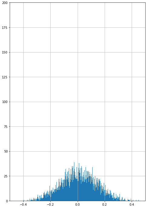
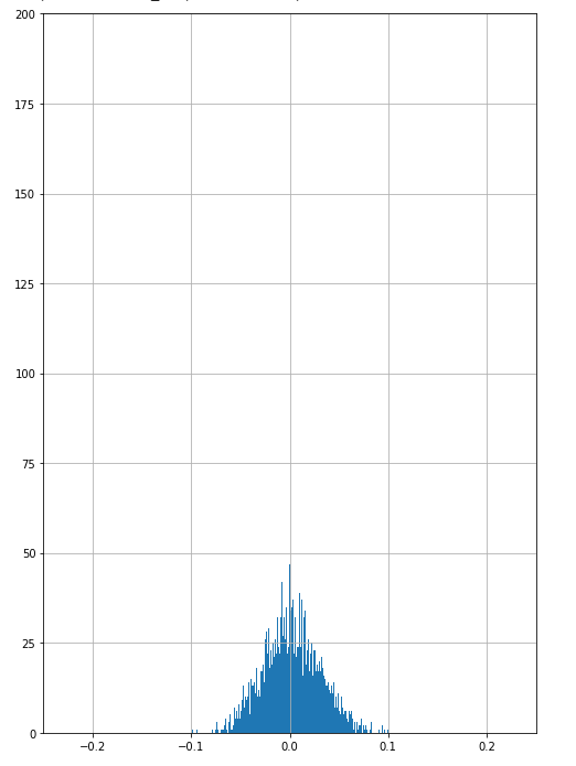
After trying conditional recurrent GANs, which didn’t train well, I tried using simpler multilayer perceptrons for both Generator and Discriminators in which I passed the entire window of returns of the adjusted close price of AAPL. The optimal window size was derived from hyperparameter tuning using Bayesian optimisation. The distribution generated by the feed-forward GAN is shown in figure 1.
Image may be NSFW. Clik here to view.
Fig 1. Returns by simple feed-forward GAN
Some of the common problems I faced were either partial or complete mode collapse - where the distribution either did not have a similar sharp peak as the empirical distribution ( partial ) or any noise sample input into the generator produces a limited set of output samples ( complete).
Image may be NSFW. Clik here to view.
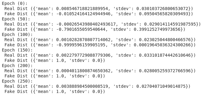
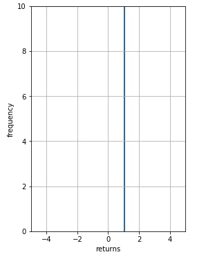
The figure above shows mode collapsing during training. Every subsequent epoch of the training is printed with the mean and standard deviation of both the empirical subset (“real data”) that is put into the discriminator for training and the subset generated by the generator ( “fake data”). As we can see at the 150th epoch, the distribution of the generated “fake data” absolutely collapses. The mean becomes 1.0 and the stdev becomes 0. What this means is that all the noise samples put into the generator are producing the same output! This phenomenon is called Mode Collapse as the frequencies of other local modes are not inline with the real distribution. As you can see in the figure below, this is the final distribution generated in the training iterations shown above:
Image may be NSFW. Clik here to view.
A few tweaks which reduced errors for both Generator and Discriminator were 1) using a different learning rate for both the neural networks. Informally, the discriminator learning rate should be one order higher than the one for the generator. 2) Instead of using fixed labels like 1 or a 0 (where 1 means “real data” and 0 means “fake data”) for training the discriminator it helps to subtract a small noise from the label 1 and add a similar small noise to label 0. This has the effect of changing from classification to a regression model, using mean square error loss instead of binary cross-entropy as the objective function. Nonetheless, these tweaks have not eliminated completely the suboptimality and mode collapse problems associated with recurrent networks.
Baseline Comparisons
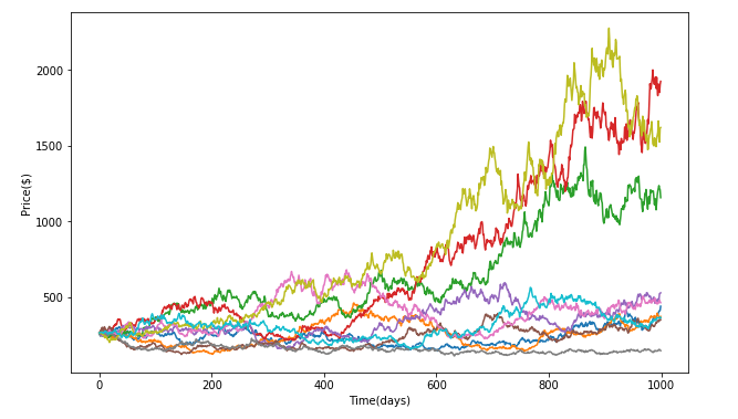
We compared this generated distribution against the distribution of empirical returns and the distribution generated via the Geometric Brownian Motion - Monte Carlo simulations done on AAPL via python. The metrics used to compare the empirical returns from GBM-MC and GAN were Kullback-Leibler divergence to compare the “distance” between return distributions and VAR measures to understand the risk being inferred for each kind of simulation. The chains generated by the GBM-MC can be seen in fig. 4. Ten paths were simulated in 1000 days in the future based on the inputs of the variance and mean of the AAPL stock data from the 1980s to 2019. The input for the initial price in GBM was the AAPL price on day one.
Image may be NSFW. Clik here to view.Image may be NSFW. Clik here to view.
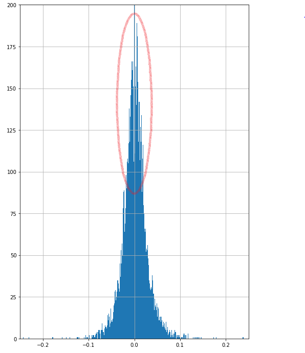
Fig 2. shows the empirical distributions for AAPL starting 1980s up till now. Fig 3. shows the generated returns by Geometric Brownian motion on AAPL.
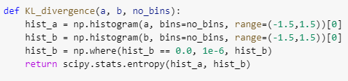
To compare the various distributions generated in the exercise I binned the return values into 10,000 bins and then calculated the Divergence using the non-normalised frequency value of each bin. The code is:
Image may be NSFW. Clik here to view.
The formula scipy uses behind the scene for entropy is:
S = sum(pk * log(pk / qk)) where pk,qk are bin frequencies
The Kullback-Leibler divergence which was calculated between distributions:
Comparison
KL Divergence
Empirical vs GAN
7.155841564194154
GAN vs Empirical
10.180867728820251
Empirical vs GBM
1.9944835997277586
GBM vs Empirical
2.990622397328334
The Geometric Brownian Motion generation is a better match for the empirical data compared to the one generated using Multiperceptron GANs even though it should be noted that both are extremely bad.
The VAR values ( calculated over 8 samples ) here tell us that beyond a confidence level, the kind of returns (or losses) we might get - in this case, it is the percentage losses with 5% and 1% chance given the distributions of returns:
Comparison
Mean and Std Dev of VAR Values ( for 95% confidence level )
Mean and Std Dev of VAR Values ( for 99% confidence level )
GANs
Mean = -0.1965352900
Stdev = 0.007326252
Mean = -0.27456501573
Stdev = 0.0093324205
GBM with Monte Carlo
Mean = -0.0457949236
Stdev = 0.0003046359
Mean = -0.0628570539
Stdev = 0.0008578205
Empirical data
-0.0416606773394755 (one ground truth value)
-0.0711425634927405 (one ground truth value)
The GBM generator VARs seem to be much closer to the VARs of the Empirical distribution.
Image may be NSFW. Clik here to view.
. Fig 4. Showing the various paths generated by the Geometric Brownian motion model using monte Carlo.
Conclusion
The distributions generated by both methods didn’t generate the sharp peak shown in the empirical distribution (figure 2). The spread of the return distribution by the GBM with Monte Carlo was much closer to reality as shown by the VAR values and its distance to the empirical distribution was much closer to the empirical distribution as shown by the Kulback-Leibler divergence, compared to the ones generated by the various GANs I tried. This exercise reinforced that GANs even though enticing are tough to train. While at it I discovered and read about a few tweaks that might be helpful in GAN training. Some of the common problems I faced were 1) mode collapse discussed above 2) Another one was the saturation of the generator and “overpowering” by the discriminator. This saturation causes suboptimal learning of distribution probabilities by the GAN. Although not really successful, this exercise creates scope for exploring the various newer GAN architectures, in addition to the conditional recurrent and multilayer perceptron ones which I tried, and use their fabled ability to learn the subtlest of distributions and apply them for financial time-series modelling. Our codes can be found at Github here. Any modifications to the codes that can help improve performance are most welcome!
About Author:
Akshay Nautiyal is a Quantitative Analyst at Quantinsti, working at the confluence of Machine Learning and Finance. QuantInsti is a premium institute in Algorithmic & Quantitative Trading with instructor-led and self-study learning programs. For example, there is an interactivecourse on using Machine Learning in Finance Markets that provides hands-on training in complex concepts like LSTM, RNN, cross validation and hyper parameter tuning.
The monthly US nonfarm payroll (NFP) announcement by the United States Bureau of Labor Statistics (BLS) is one of the most closely watched economic indicators, for economists and investors alike. (When I was teaching a class at a well-known proprietary trading firm, the traders suddenly ran out of the classroom to their desks on a Friday morning just before 8:30am EST.) Naturally, there were many efforts in the past trying to predict this number, ranging from using other macroeconomic indicators such as credit spreads to using Twitter sentiment as predictive features. In this article, I will report on research conducted by Radu Ciobanu and I using the unique and proprietary continuous survey data provided by RIWI Corp.to predict this important number.
RIWI is an alternative data provider that conducts online surveys and risk measurement monitoring in all countries of the world anonymously, without collecting any personally identifiable information or providing incentives to respondents. RIWI’s technology has collected and analyzed more than 1.5 billion responses globally. Critically, in their surveys, they can reach a segment of the population that is usually hidden: three quarters of their respondents across the world have not answered a survey of any kind in the preceding month. Their surveys strive to be as representative of the general online population as possible, without the usual bias towards the loud social media voices. This is important in predictive data for financial markets, where it is vital to separate noise from signal.
The financial market reacts mainly to surprise, i.e. the difference between the actual announced NFP number and the Wall Street consensus. This surprise can move not only the US financial markets, but international markets as well. Case in point: I watched the German DAX index moved sharply higher last week (December 6, 2019 ) due to the huge positive surprise (adding 266K jobs instead of the Wall Street consensus of 183K).Therefore the surprise is what we want to predict. We compared predicting the sign of this surprise using machine learning with the RIWI score as the only feature vs. a number of other benchmarks that do not include the RIWI score, and found that the RIWI score generates higher predictive accuracy than all other benchmarks during cross validation test. We also predicted both the magnitude and sign of the NFP surprise. Including the RIWI score as one of the features achieved the smallest averaged cross-validated mean squared error (MSE) than otherwise. Limited out-of-sample results indicate the RIWI score continues to have significant power for both sign and magnitude predictions.
Data
The historical NFP monthly numbers were seasonally adjusted by the BLS. These numbers were released on the first Friday of every month, at 8:30 am ET (except on certain national holidays when they are released one day before or delayed by one week.) To compute the surprise, we subtract the Wall Street consensus on the day before the announcement from the actual NFP number.
The RIWI data were based on their online surveys of US consumers, and consist of two datasets. The first one is dated December 2013 - October 2017 and the second one is dated Sep 2018 - Sep 2019. The former dataset is based on the yes/no answer to the following survey question: ‘Are you working for more than 35 hours per week?’. The latter dataset is based on several survey questions related to opinions regarding US companies or products, along with respondents’ personal background, such as their employment status (full-time/part-time/student/retired), marital status, etc. In order to merge the two datasets, we regard respondents who said they worked “full-time” or “part-time” as equivalent to “working more than 35 hours per week”. If we were to count only the “full-time” respondents, a significant structural break in the time series would be observed between the two time periods, as seen in Figure 1 below.
Figure 1: Weighted monthly RIWI score, without seasonal adjustments, including only “Full-Time” respondents, for Dec 2013-Oct 2017 and Sep 2018-Sep 2019.
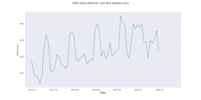
If we include both “Full-time” and “Part-Time” respondents, we obtain Figure 2 below, which clearly doesn’t have that structural break.
Figure 2: Weighted monthly RIWI score, without seasonal adjustments, including “Full-time + part-time” respondents, for Dec 2013-Oct 2017 and Sep 2018-Sep 2019.
RIWI provides a weight for each respondent in order to transform the data so that it can reflect the demographics of the general US population, hence the adjective “Weighted” in the figure captions. Note that the survey is conducted such that each respondent can go back and change their answers but they will not show up as more than one sample in the data set. In order to extract a summary score in advance of each month’s NFP announcement, we compute a monthly average of the product of the respondents’ weights and the indicator (0 or 1) of whether the individual respondent is working full or part-time. The monthly average is computed over the same month that the NFP number measures. We call this the “RIWI score”. As the NFP data were seasonally adjusted, we need to do the same to the monthly differences of the RIWI score. We employ the same adjustment that the BLS uses: X12-ARIMA. But for comparison purposes, we did not apply seasonal adjustment to Figures 1 and 2.
Classification models
Our classification models were used to predict whether the sign of the NFP surprisewas positive or negative (there were no zero surprises in the data.) The models were trained on the data on Dec 2013 – Oct 2017 (“train set”), where cross validation testing also took place. Out-of-sample testing was done on the data Sep 2018-Oct 2019 (“test set”). As mentioned above, the test set’s RIWI survey questions were somewhat different from the train set questions. So test set result is a joint test of whether the classification model works out-of-sample and whether the slight difference in the RIWI data degrades predictive accuracy significantly.
To provide benchmark comparisons against RIWI score, we also studied several other standard features, some of which were found useful for NFP predictions:
·Previous 1-month NFP surprise
·Previous 12-month NFP surprise
·BloombergBarclays US Corporate High Yield Average Option Adjusted Spread Index (a.k.a. credit spreads)
·Index of Consumer Sentiment (University of Michigan)
The Bloomberg Barclays US Corporate High Yield Average Option Adjusted SpreadIndex denotes the difference (spread) between a computed Option Adjusted Spread index of all high yield corporate bonds and a spot US Treasury curve. An Option Adjusted Spread index is computed using constituent bonds’ option adjusted spreads, weighted by market capitalization. In what follows, we will refer to the Bloomberg Barclays US Corporate High Yield Average Option Adjusted Spread Index as the “credit spreads” feature.
Since machine learning can only be performed on stationary features, we will use the monthly differences in the RIWI score and other features.
The benchmarks models we tested are:
Logistic regression* on Previous surprise.
Trend-following model predicts next sign(surprise)=sign(previous surprise).
Contrarian model predicts next sign(surprise)=-sign(previous surprise).
Logistic regression on credit spreads.
Logistic regression on Index of Consumer Sentiment.
*All logistic regressions were L2-regularized.
Here are the results, compared to applying Random Forest to the RIWI score alone:
ML model
Features
CV accuracy (in-sample)
Out-of-sample accuracy
Contrarian model
Prev 1-month surprise
0.46
0.66
LogReg (Ridge)
Credit spreads
0.52
0.51
LogReg (Ridge)
Prev 1-month surprise
0.53
0.50
LogReg (Ridge)
Consumer sentiment index
0.53
0.50
Random Forest
All features
0.53
0.58
Trend following model
Prev 1-month surprise
0.54
0.33
Random Forest
RIWI score alone
0.63+/- 0.03
0.58+/- 0.04
Table 1: Classification benchmarks and other features
Based on the predictive accuracy on the cross validation data, the best machine learning model is one that uses the RIWI score as the onlyfeature. This model applied the random forest classifier to the RIWI score to predict sign(NFP surprise). It obtained an average cross-validated (CV) accuracy of 63% +/- 0.03 (using 10-fold cross-validation on Dec 2013 – Oct 2017 data) and a 58.3% +/- 0.04 out-of-sample accuracy. As the out-of-sample data consists only of 12 data points, we view that as a test of whether the random forest classifier overfitted on training data, and whether the slightly different RIWI data affected predictions, but not as a fair comparison of the various models. Since the predictive accuracy did not deteriorate significantly on the out-of-sample data, we conclude that no overfitting was likely, and the new RIWI data did not differ significantly from that which we trained on. We have also applied random forest to all the features including the RIWI score, and found lower CV (53%) and out-of-sample (58%)accuracies than using the RIWI score alone.
Regression models
Our regression models were used to predict the actual NFP surprise (sign + magnitude). The train vs. test data were the same as for the classification models, and features set were also the same.
To provide benchmark comparisons against the RIWI score, we studied the following models:
ARMA (2,1) model* that uses past NFP surprises.
Trend-following model predicts next surprise=(previous surprise).
Contrarian model predicts next surprise=-(previous surprise).
*The lags and coefficients were optimized based on AIC minimization on the train set.
Here are the results, compared to applying Random Forest to the RIWI score alone:
Based on the mean squared error (MSE) of predicted surprises on the cross validation data, the best machine learning model is one that includesthe RIWI score as a feature. It applied the random forest classifier to the RIWI score, previous 1-month and 12-month surprises in order to predict actual NFP surprise. It obtained an average cross-validated MSE of 3249.35 +/- 70 and a 7269.2+/- 134 out-of-sample accuracy. It marginally outperformed all benchmarks in cross-validation. As with all other benchmarks, including the Contrarian model which requires no training, out-of-sample MSE increased significantly over the CV MSE. But again, as the out-of-sample data consists only of 12 data points, we don’t view it as a fair comparison of the various models. We also applied random forest to all the features including the RIWI score, and found somewhat higher CV MSE (and hence a worse model) than using the RIWI score alone, but the difference is within error bounds.
Conclusion and Future Work
Using the technique of cross validation on RIWI data from December 2013 - October 2017, we found that the RIWI score (after weighting, seasonal adjustment, and differentiation), has outperformed all other benchmarks in predictive accuracy for the sign of the NFP surprises. We also found that the similarly transformed RIWI score, if supplemented with other indicators, has performed as well or better than all other benchmarks. While such absolute dominance needs to be confirmed in an extended out-of-sample test, we believe there is great potential for using the RIWI score for predicting the all-important Nonfarm Payroll number.
But beyond predicting NFP surprises, RIWI’s data have the potential to be a more accurate gauge of the actual U.S. employment situation, and therefore economic growth, than the NFP number. The “gig economy” is employing more workers whose data do not easily find their way into the official BLS count. (Here is an articleon why BLS’ effort to count these workers has been a failure. This Bank of Canada reportalso concluded that official numbers were undercounting gig workers.) Undocumented workers are not counted in the NFP but they do contribute to the economy. Even illegal activities could have contributed more than 1% to the U.S. GDP, according to this Wall Street Journal report. In contrast, RIWI’s survey methodology was cited in this paperby Harvard researchers among others as the preferred method of collecting data on hard-to-reach populations. One can imagine an ambitious researcher using RIWI data to directly predict GDP growth and achieving better results than using the traditional economic indicators such as NFP.
Acknowledgement
We thank Jason Cho, Head of Data Operations at RIWI, for providing us the Company’s proprietary data for our evaluation purposes.
*Note a PDF version of this article can be downloaded from www.epchan.com.
I generally don't like to write about our investment programs here, since the good folks at the National Futures Association would then have to review my blog posts during their regular audits/examinations of our CPO/CTA. But given the extraordinary market condition we are experiencing, our kind cap intro broker urged me to do so. Hopefully there is enough financial insights here to benefit those who do not wish to invest with us.
As the name of our Tail Reaper program implies, it is designed to benefit from tail events. It did so (+20.07%) during August-December, 2015’s Chinese stock market crash (even though it trades only the E-mini S&P 500 index futures), it did so (+18.38%) during February-March, 2018’s “volmageddon”, and now it did it again (+12.98%) during February, 2020’s Covid-19 crisis. (As of this writing, March is up over 21% gross.) There are many names to this strategy: some call it “crisis alpha”, others call it “convex”, “long gamma” or “long vega” (even though no options are involved), “long volatility”, “tail hedge”, or just plain old “trend-following”. Whatever the name or description, it usually enjoys outsize return when there is real panic. (But of course, PAST PERFORMANCE IS NOT NECESSARILY INDICATIVE OF FUTURE RESULTS.) Furthermore, our strategy did so without holding any overnight positions.
Why is a trend-following strategy profitable in a crisis? A simple example will suffice. If a short trade is triggered when the return (from some chosen benchmark) exceeds -1%, then the trade will be very profitable if the market ends up dropping -4%. Vice versa for a long trade. (As recent market actions have demonstrated, prices exhibit both left and right tail movements in a crisis.) The trick, of course, is to find the right benchmark for the entry, and to find the right exit condition.
Naturally, insurance against market crash isn’t completely free. Our goal is to prevent the insurance cost, which is essentially the loss that the strategy suffers during a stretch of bull market, from being too high. After all, if insurance were all we want, we could have just bought put options on the market index, and watched it lost premium every month in “good” times. To prevent the loss of insurance premium requires a dose of market timing, assisted by our machine learning program that utilizes many, many factors to predict whether the market will suffer extreme movements in the next day. In most years, the cost (loss) is negligible despite the long bull market, except in 2019 when we lost 8.13%. That year, which seems a long time ago, the SPY was up 30.9%. (It was in the August of that year that we added the machine learning risk management layer.) But most investors have a substantial long exposure. A proper asset allocation to both Tail Reaper and to a long-only portfolio will smooth out the annual returns and hopefully eliminate any losing year. (Again, PAST PERFORMANCE IS NOT NECESSARILY INDICATIVE OF FUTURE RESULTS.)
But why should we worry about a losing year? Isnt’ total return all investors should care about? Recently, Mark Spitznagel (who co-founded Empirica Capital with Nassim Nicholas Taleb) wrote a series of interesting articles. It argued that even if a tail hedge strategy like ours returns an arithmetic average return of 0%, as long as it provides outsize positive returns during a market crisis, it will be able to significantly improves the compound growth rate of a portfolio that includes both an index fund and the tail hedge strategy. I have previously written a somewhat technical blog post on this mathematical curiosity. The gist of the argument is that the compound growth rate of a portfolio is m-s^2/2, where m is the arithmetic mean return and s is the standard deviation of returns. Hedging tail risk is not just for the psychological comfort of having no losing years - it is mathematically proven to improve long-term compound growth rate overall.
PAST PERFORMANCE IS NOT NECESSARILY INDICATIVE OF FUTURE RESULTS.
For further reading on convex strategies, please see the papers by Paul Jusselin et al “Understanding the Momentum Risk Premium: An In-Depth Journey Through Trend-Following Strategies” and Dao et al “Tail protection for long investors: Trend convexity at work” (Hat tip to Corey Hoffstein for leading me to them!)
What is the probability of profit of your next trade? You would think every trader can answer this simple question. Say you look at your historical trades (live or backtest) and count the winners and losers, and come up with a percentage of winning trades, say 60%. Is the probability of profit of your next trade 0.6? This might be a good initial estimate, but it is also a completely useless number. Let me explain.
This 0.6 is what may be called an unconditional probability of profit. It is the same for every trade that you will ever make (unless your winning ratio changes significantly in the future), so it is useless as a guide to whether you should take the next specific trade or not. It can of course tell you whether you should trade this strategy in general (e.g. you may not want to trade a strategy with an unconditional probability of profit, a.k.a. winning ratio, less than 0.51). But it can’t do so on a trade-by-trade basis. The latter is the conditional probability of profit. As the adjective suggests, this probability is conditioned on the specific market environment at the time when you expect to trade.
Let's say you are trading a short volatility strategy. It can be an algorithmic, or even discretionary, strategy. If you are trading it during a very calm market, it is likely that your conditional probability of profit would be quite high. If you are trading during a financial crisis, it could be very low. The conditions that can determine the probability may even be quantifiable. The level of VIX? The recent SPY returns? How about the interest rate change or Nonfarm Payroll number just announced? Or even the % change in Covid-19 cases on the previous day? You may not have taken all these myriad numbers into account when you were building your simple trading strategy, or when you decide to make a discretionary trade, but you can't deny they may have an impact on the conditional probability of profit. So how are we to compute this probability?
Spoiler alert: computing this conditional probability helped us earned 64% YTD return as of June 2020. You can find out how to do that with predictnow.ai. But more on that later.
The only known way to compute this conditional probability is machine learning. Let's return to the example of your short volatility strategy above. Suppose you prepare a spreadsheet of the returns of the historical trades you have done, like this:
Image may be NSFW. Clik here to view.
Figure 1: Spreadsheet with historical returns of short vol trades.
Again, these trades could be due to an algorithm, or it could be discretionary (perhaps based on some combination of fundamental analysis and intuition like what Warren Buffet does).
Now let's say we only care about whether they are profitable or not, so we ignore the magnitude of returns and label those trades that are profitable 1, otherwise 0. (These are called "metalabels" by Marcos Lopez de Prado, who pioneered this financial machine learning technique. They are “meta” because he assumed the original simple strategy is used to predict the ups and downs of the market itself – those are the base predictions, or labels. The metalabels are on whether those base predictions are correct or not.) The resulting spreadsheet looks like this.
Image may be NSFW. Clik here to view.
Figure 2: Spreadsheet with labels: are historical returns of short vol strategy profitable?
Simple, right? Now comes the hard part. Your intuition tells you that there are some variables that you didn't take into account in your original, simple, trading strategy. There are just too many of these variables, and you don't know how to incorporate them to improve your trading strategy. You don't even know if some of them are useless. But that's not a problem for machine learning. You can add as many variables, called features / predictors / independent variables, as you like, useful or not. The machine learning algorithm will get rid of the useless features via a process called feature selection. But more on that later.
So let's say for every historical trade (represented by a row in the spreadsheet), you collect some features like VIX, 1-day SPY return, change in interest rate on the previous day, etc. We must, of course, ensure that these features' values were known prior to each trade's entry time, otherwise there will be look-ahead bias and you won't be able to use this system for live trading. So here is how your spreadsheet augmented with features may look:
Image may be NSFW. Clik here to view.
Figure 3: Spreadsheet with features augmented.
OK, now that you have prepared all these historical data, how do you build (or "train", in machine learning parlance) a predictive model based on that? You may not know it, but you have probably used the simplest kind of machine learning model already, maybe way back in a college statistics class. It is called linear regression, or its close sibling logistic regression for our binary (profit or not) classification problem. Those features that you created above are just the independent variables, often called X (a vector of many variables), and the labels are just the dependent variable often called Y (with values of 0 or 1). But applying linear or logistic regression on a large, disparate set of features to predict a label usually fails, because many relationships cannot be captured by a linear model. The nonlinear co-dependences between these predictors need to be discovered and utilized. For example, maybe when VIX <= 15, the 1-day SPY return isn't useful for predicting the probability of profit of your trade. But when VIX >= 15, 1-day SPY return is very useful. This type of relationship is best discovered using a "supervised" hierarchical learning algorithm called random forest, which is what we have implemented on predictnow.ai.
A random forest algorithm may discover the hypothetical relationship between VIX, 1-day SPY return, …, and whether your short vol trade will be profitable as illustrated in this schematic diagram:
Figure 4: Example classification tree generated by predictnow.ai internally.
To build this tree, and all its cousins that together form a "random forest", all you need to do is to upload your spreadsheet above to predictnow.ai, click a button, and it will probably be done in less than 15 minutes, often much sooner. (Certainly faster than a pizza delivery.)
Image may be NSFW. Clik here to view.
Figure 5: Choosing training mode at predictnow.ai.
Image may be NSFW. Clik here to view.
Figure 6: Uploading training data.
Image may be NSFW. Clik here to view.
Figure 7: Choosing hyperparameters for building random forest.
Once this random forest is built (trained) with historical data, it is ready for your live trading. You can just plug in the latest values for VIX, 1-day SPY, and any other features into a new spreadsheet like this:
Image may be NSFW. Clik here to view.
Figure 8: Live trading input.
Notice that the format of this spreadsheet is the same as the training data, except that there is no known Return of course - we are hoping to predict that! You can upload this to predictnow.ai together with the model you just trained, press PREDICT,
Image may be NSFW. Clik here to view.
Figure 9: Live prediction.
and voila! You can now download the random forest's prediction of whether that trade will be profitable, and with what conditional probability.
One of the output files (left in Figure 10) tells you the most likely outcome of your trade: profit or not. The other file (right one in Figure 10) tells you the probability of that outcome. You can use that probability to size your trade. For example, you may decide that if the probability of profit is higher than 0.6, you will buy $10K of TSLA. But if the probability is between 0.51 and 0.6, you will only buy $5K, while if the probability is lower than 0.51, you won’t buy at all.
Typically the live prediction will take 1 second or less, while the training (which may not need to be re-done more than once a quarter) typically won't take more than 15 minutes even for thousands of rows of historical data with 100 features. You can make live predictions as frequently as you like (i.e. as frequently as your input changes), but if you are a high frequency trader, you would want to use our API so that our predictions can be seamlessly integrated with your trading system.
But predicting the conditional probability of profit for your next trade is not all that we can do. We can also tell you what features are important in making that prediction. In fact, you may be more interested in that than a black-box prediction, because this list of important features, sorted in decreasing order of importance, may help you improve your underlying simple trading strategy. In other words, it can help improves your intuition about what works with your strategy, so you can change your trading rules.
Going back to our example, predictnow.ai can generate such a graph for you:
You can see that VIX was deemed the most important feature, followed by 1-day SPY return, the latest interest rate change, and so on. Our internal predictive algorithm will actually remove all features that are "below average" and retrain the model, but you may benefit from incorporating just VIX and 1-day SPY return in your simple strategy when it generates a trading signal. Remember, your simple strategy does not need to be an algorithmic strategy. It could be discretionary.
(For the machine learning mavens among you, we use SHAP for feature selection, as discussed in our paper.)
You may wonder why our predictive service is restricted to only taking your strategy’s historical or live trades as input and predicting their probabilities of profit. Why can’t it be used directly to predict the market’s return? Of course it can: you only need to pretend that your strategy is buy-and-holding the market. It can even predict the magnitude, not just the sign, of the return. But as we all know, it is very hard to predict the market’s movement, because of low signal-to-noise ratio. Your own strategy, however, has presumably found a way to filter out those noise, and machine learning prediction is more likely to succeed in telling you what “regime” is favorable/unfavorable to your strategy, and with what probability. Another usage of our service is to use it to predict numbers that are not subject to arbitrage, things such as a company’s earning surprise, credit rating change, or the US nonfarm payroll surprise (as we have already done successfully). In these usages, there are no adversaries (your fellow traders) that are trying their hardest to arbitrage away your trading alpha, so these predictions will be more likely to work far into the future.
(For machine learning mavens, you may wonder why we have only implemented random forest learning algorithm. The beauty of random forest is that it is simple, but not too simple. Complicated deep learning algorithms such as LSTM can indeed take into account the time series dependence of the features and labels more readily, but they run serious risk of data snooping due to the large number of parameters to fit. GPT-3, the latest and hottest deep learning algorithm for natural language processing, for example, has more than 175 billion parameters to fit. Imagine fitting that to 1,000 historical trades!)
So does this stuff really work? We have implemented this machine learning system for our Tail Reaper strategy in our fund around the August of 2019. Yes, the 64% YTD return as of June 2020 (net of 25% incentive fee!) is nice, but what's more amazing is that the machine learning program told us to not enter any trade (due to the low conditional probability of profit) from Nov 2019 - Jan 2020. In retrospect, that made sense because Tail Reaper is a crisis alpha, tail hedge strategy. There was no crisis, no tail movement, from which to reap profits in those calm months. But suddenly, starting on February 1, 2020, this machine learning program told us to expect a crisis. We thought the machine learning program was nuts - there were just a handful of Covid-19 cases in the US at that time! Nonetheless we followed its advice and restarted Tail Reaper. It went on to capture over 12% return later that month, and the rest is history. (Past performance is not necessarily indicative of future results. For detailed disclosure of this strategy, please visit qtscm.com.)
Image may be NSFW. Clik here to view.
Figure 12: Tail Reaper equity curve.
For readers interested in a free trial or to participate in a live webinar on how to use predictnow.ai to predict the conditional probability of profit of your trades, please sign up here.
One major impediment to widespread adoption of machine learning (ML) in investment management is their black-box nature: how would you explain to an investor why the machine makes a certain prediction? What's the intuition behind a certain ML trading strategy? How would you explain a major drawdown? This lack of "interpretability" is not just a problem for financial ML, it is a prevalent issue in applying ML to any domain. If you don’t understand the underlying mechanisms of a predictive model, you may not trust its predictions.
Feature importance ranking goes a long way towards providing better interpretability to ML models. The feature importance score indicates how much information a feature contributes when building a supervised learning model. The importance score is calculated for each feature in the dataset, allowing the features to be ranked. The investor can therefore see the most important predictors (features) used in the predictions, and in fact apply "feature selection" to only include those important features in the predictive model. However, as my colleague Nancy Xin Man and I have demonstrated in Man and Chan 2021a, common feature selection algorithms (e.g. MDA, LIME, SHAP) can exhibit high variability in the importance rankings of features: different random seeds often produce vastly different importance rankings. For e.g. if we run MDA on some cross validation set multiple times with different seeds, it is possible that a feature in a run is ranked at the top of the list but dropped to the bottom in the next run. This variability of course eliminates any interpretability benefit of feature selection. Interestingly, despite this variability in importance ranking, feature selection still generally improves out-of-sample predictive performance on multiple data sets that we tested in the above paper. This may be due to the "substitution effect": many alternative (substitute) features can be used to build predictive models with similar predictive power. (In linear regression, substitution effect is called "collinearity".)
To reduce variability (or what we called instability) in feature importance rankings and to improve interpretability, we found that LIME is generally preferable to SHAP, and definitely preferable to MDA. Another way to reduce instability is to increase the number of iterations during runs of the feature importance algorithms. In a typical implementation of MDA, every feature is permuted multiple times. But standard implementations of LIME and SHAP have set the number of iterations to 1 by default, which isn't conducive to stability. In LIME, each instance and its perturbed samples only fit one linear model, but we can perturb them multiple times to fit multiple linear models. In SHAP, we can permute the samples multiple times. Our experiments have shown that instability of the top ranked features do approximately converge to some minimum as the number of iterations increases; however, this minimum is not zero. So there remains some residual variability of the top ranked features, which may be attributable to the substitution effect as discussed before.
To further improve interpretability, we want to remove the residual variability. López de Prado, M. (2020) described a clustering method to cluster together features are that are similar and should receive the same importance rankings. This promises to be a great way to remove the substitution effect. In our new paper Man and Chan 2021b, we applied a hierarchical clustering methodology prior to MDA feature selection to the same data sets we studied previously. This method is generally called cMDA. As they say in social media click baits, the results will (pleasantly) surprise you.
Not only do these clusters have clear interpretations (provided by us as a "Topic"), these clusters almost never change in their top importance rankings under 100 random seeds!
Closer to our financial focus, we also applied cMDA to a public dataset with features that may be useful for predicting S&P 500 index excess monthly returns. The two clusters found are
The two clusters can clearly be interpreted as fundamental vs technical indicators, and their rankings don't change: fundamental indicators are always found to be more important than technical indicators in all 100 runs with different random seeds.
Finally, we apply this technique to our proprietary features for predicting the success of our Tail Reaper strategy. Again, the top 2 clusters are highly interpretable, and never change with random seeds. (Since these are proprietary features, we omit displaying them.)
If we select only those clearly interpretable, top clusters of features as input to training our random forest, we find that their out-of-sample predictive performances are also improved in many cases. For example, the accuracy of the S&P 500 monthly returns model improves from 0.517 to 0.583 when we use cMDA instead of MDA, while the AUC score improves from 0.716 to 0.779.
S&P 500 monthly returns prediction
F1
AUC
Acc
cMDA
0.576
0.779
0.583
MDA
0.508
0.716
0.517
Full
0.167
0.467
0.333
Meanwhile, the accuracy of the Tail Reaper metalabeling model improves from 0.529 to 0.614 when we use cMDA instead of MDA and select all clustered features with above-average importance scores, while the AUC score improves from 0.537 to 0.672.
F1
AUC
Acc
cMDA
0.658
0.672
0.614
MDA
0.602
0.537
0.529
Full
0.481
0.416
0.414
This added bonus of improved predictive performance is a by-product of capturing all the important, interpretable features, while removing most of the unimportant, uninterpretable features.
You can try out this hierarchical cluster-based feature selection for free on our financial machine learning SaaS predictnow.ai. You can use the no-code version, or ask for our API. Details of our methodology can be found here.
Tradetron.tech is a new algo strategy marketplace that allows one to build algo strategies without coding and others to subscribe to them and take trades in their own linked brokerage accounts automatically. It can handle complex strategies such as arbitrage and options strategies. Currently some 400 algos are on offer.
Jonathan Landy, a Caltech physicist, together with 3 of his physicist friends, have started a deep data science and machine learning blog with special emphasis on finance.
Every trader knows that there are market regimes that are favorable to their strategies, and other regimes that are not. Some regimes are obvious, like bull vs bear markets, calm vs choppy markets, etc. These regimes affect many strategies and portfolios (unless they are market-neutral or volatility-neutral portfolios) and are readily observable and identifiable (but perhaps not predictable). Other regimes are more subtle, and may only affect your specific strategy. Regimes may change every day, and they may not be observable. It is often not as simple as saying the market has two regimes, and we are currently in regime 2 instead of 1. For example, with respect to the profitability of your specific strategy, the market may have 5 different regimes. But it is not easy to specify exactly what those 5 regimes are, and which of the 5 we are in today, not to mention predicting which regime we will be in tomorrow. We won’t even know that there are exactly 5!
Regime changes sometimes necessitate a complete change of trading strategy (e.g. trading a mean-reverting instead of momentum strategy). Other times, traders just need to change the parameters of their existing trading strategy to adapt to a different regime. My colleagues and I at PredictNow.ai have come up with a novel way of adapting the parameters of a trading strategy, a technique we called “Conditional Parameter Optimization” (CPO). This patent-pending invention allows traders to adapt new parameters as frequently as they like—perhaps for every trading day or even every single trade.
CPO uses machine learning to place orders optimally based on changing market conditions (regimes) in any market. Traders in these markets typically already possess a basic trading strategy that decides the timing, pricing, type, and/or size of such orders. This trading strategy will usually have a small number of adjustable trading parameters. Conventionally, they are often optimized based on a fixed historical data set (“train set”). Alternatively, they may be periodically reoptimized using an expanding or rolling train set. (The latter is often called “Walk Forward Optimization”.) With a fixed train set, the trading parameters clearly cannot adapt to changing regimes. With an expanding train set, the trading parameters still cannot respond to rapidly changing market conditions because the additional data is but a small fraction of the existing train set. Even with a rolling train set, there is no evidence that the parameters optimized in the most recent historical period gives better out-of-sample performance. A too-small rolling train set will also give unstable and unreliable predictive results given the lack of statistical significance. All these conventional optimization procedures can be called unconditional parameter optimization, as the trading parameters do not intelligently respond to rapidly changing market conditions. Ideally, we would like trading parameters that are much more sensitive to the market conditions and yet are trained on a large enough amount of data.
To address this adaptability problem, we apply a supervised machine learning algorithm (specifically, random forest with boosting) to learn from a large predictor (“feature”) set that captures various aspects of the prevailing market conditions, together with specific values of the trading parameters, to predict the outcome of the trading strategy. (An example outcome is the strategy’s future one-day return.) Once such machine-learning model is trained to predict the outcome, we can apply it to live trading by feeding in the features that represent the latest market conditions as well as various combinations of the trading parameters. The set of parameters that results in the optimal predicted outcome (e.g., the highest future one-day return) will be selected as optimal, and will be adopted for the trading strategy for the next period. The trader can make such predictions and adjust the trading strategy as frequently as needed to respond to rapidly changing market conditions.
In the example you can download here, I illustrate how we apply CPO using PredictNow.ai’s financial machine learning API to adapt the parameters of a Bollinger Band-based mean reversion strategy on GLD (the gold ETF) and obtain superior results which I highlight here:
Unconditional Optimization
Conditional Optimization
Annual Return
17.29%
19.77%
Sharpe Ratio
1.947
2.325
Calmar Ratio
0.984
1.454
The CPO technique is useful in industry verticals other than finance as well – after all, optimization under time varying and stochastic condition is a very general problem. For example, wait times in a hospital emergency room may be minimized by optimizing various parameters, such as staffing level, equipment and supplies readiness, discharge rate, etc. Current state-of-the-art methods generally find the optimal parameters by looking at what worked best on average in the past. There is also no mathematical function that exactly determines wait time based on these parameters. The CPO technique employs other variables such as time of day, day of week, season, weather, whether there are recent mass events, etc. to predict the wait time under various parameter combinations, and thereby find the optimal combination under the current conditions in order to achieve the shortest wait time.
We can provide you with the scripts to run CPO on your own strategy using Predictnow.ai’s API. Please email info@predictnow.ai for a free trial.
Features are inputs to supervised machine learning (ML) models. In traditional finance, they are typically called “factors”, and they are used in linear regression models to either explain or predict returns. In the former usage, the factors are contemporaneous with the target returns, while in the latter the factors must be from a prior period.
There are generally two types of factors: cross-sectional vs time-series. If you are modeling stock returns, cross-sectional factors are variables that are specific to an individual stock, such as its earnings yield, dividend yield, etc. In our previous blog post, we described how we provide 40 such factors to our subscribers for backtesting and live predictions. But as we advocate using ML for risk management and capital allocation purposes (i.e. metalabeling), not for returns predictions, you may wonder how these factors can help predict the returns of your trading strategy or portfolio. For example, if you have a long-short portfolio of tech stocks such as AAPL, GOOG, AMZN, etc., and want to predict whether the portfolio as a whole will be profitable in a certain market regime, does it really make sense to have the earnings yields of AAPL, GOOG, and AMZN as individual features?
Meanwhile, time-series factors are typically market-wide or macroeconomic variables such as the familiar Fama-French 3-factors:market (simply, the market index return), SMB (the relative return of small cap vs large cap stocks), and HML (the relative return of value vs growth stocks). These time-series factors are eminently suitable for metalabeling, because they can be used to predict your portfolio or strategy’s returns.
Given that there are many more obvious cross-sectional factors than time-series factors available, it seems a pity that we cannot use cross-sectional factors as features for metalabeling. Actually, we can – Eugene Fama and Ken French themselves showed us how. If we have a cross-sectional factor on a stock, all we need to do is to use it to rank the stocks, form a long-short portfolio using the rankings, and use the returns of this portfolio as a time-series factor. The long-short portfolio is called a hedge portfolio.
We show the process of creation of a hedge portfolio with the help of an example, starting with Sharadar’s fundamental cross-sectional factors (which we generated as shown in the blog). There are 40 cross sectional factors updated at three different frequencies - quarterly, yearly and twelve month trailing. In this exercise, however, we use only the quarterly cross-sectional factors. Given a factor like capex (capital expenditure), we consider the normalized (the normalization procedure is found in the previously cited blog post) capex of approximately 8500 stocks on particular dates from January 1st, 2010 till current date. There are 4 particular dates of interest every year -January 15th, April 15th, July 15th and October 15th. We call these the ranking dates. On each of these dates we find the percentile rank of the stock based on normalized capex. The dates are carefully chosen to capture change in the cross sectional factors of the maximum number of stocks post the quarterly filings.
Once the capex across stocks is ranked at each ranking date (4 dates) each year we obtain the stocks present in the upper quartile (i.e ranked above 75 percentile) and the stocks present in the lower quartile (i.e ranked below 25 percentile). We take a long position on the ones which showed highest normalized capex and take a short position on the ones with the lowest. Both these sets together make our long-short hedge portfolio.
Once we have the portfolio on a given ranking date we generate the daily returns of the portfolio using risk parity allocation (i.e allocate proportional to inverse volatility). The daily returns of each chosen stock are calculated for each day till the next ranking date. The portfolio weights on each day are the normalized inverse of the rolling standard deviation of returns for a two month window. These weights change on a daily basis and are multiplied to the daily returns of individual stocks to get the daily portfolio returns.If a portfolio stock is delisted in between ranking dates we simply drop the stock and not use it to calculate the portfolio returns. The daily returns generated in this process are the capex time series factors. This process is repeated for all other Sharadar cross-sectional factors.
So, voila! 40 cross-sectional factors become 40 time-series factors, and they can be used for metalabeling any portfolio or trading strategy, whether it trades stocks, futures, FX, or anything at all.
What about the opposite conversion? Can we turn time-series factors into cross-sectional factors suitable for predicting the returns of individual stocks? Actually, there is no need. You can directly add any time-series factor to your feature set for predicting individual stock’s returns. This is equivalent to building a linear factor model with an individual stock’s returns as dependent variable and the time-series factor as independent variable, a process well-known in traditional finance.
On a side note: besides these 40 time-series (and their corresponding cross-sectional) features, we have compiled an additional 197 proprietary time-series features available to our Premium subscribers, and available via our API.
This has been a summer of feature engineering for PredictNow.ai. First, we launched the US stock cross-sectional features and the time-series market-wide features. Now we have launched the features based on options activities, ETFs, futures, and macroeconomic indicators. In total, we are now offering 616 ready-made features to our subscribers.
There is a lot to read here. If you would rather join our October 1, 12pm EST webinar where Ernie and I will discuss these factors / features and answer your questions, please sign up here.
NOPE - Net options pricing effect - is a normalized measure of the net delta imbalance between the put and call options of a traded instrument across its entire option chain, calculated at the market close for contracts of all maturities. This indicator was invented by Lily Francus (Twitter: @nope_its_lily) and is normalized with the total traded volume of the underlying instrument. The imbalance estimates the amount of delta hedging by market markers needed to keep their positions delta-neutral. This hedging causes price movement in the underlying, which NOPE should ideally capture. The data for this has been sourced from Delta Neutral.and the instrument we applied it to was SPY ETF options. The SPX index options were’t used because the daily traded volume of the underlying SPX index “stock” was irrational. It was calculated as the traded volume of the constituents of the index.
Canary - is an indicator that acts similar to a canary in a coal mine, which will raise an alarm when there’s an impending danger. This indicator comes from the dual momentum strategies of Vigilant and Defensive Asset allocation. The canary value can be either 0,1 or 2. This is a daily measure of which of the two bond or stock ETFs has a negative absolute momentum - 1) BND - Vanguard Total Bond Market ETF 2) VMO - Vanguard Emerging Markets Stock Index Fund ETF. The momentum is calculated using the 13612W method where we take a proportionally weighted average of percentage change in the bond/stock ETF returns in the last 1 month, 3 months, 6 months, and 1 year. In the paper, the values of “0”,”1” or “2” of the canary portfolio represent what percentage of the canary is bullish. This indicates what proportion of the asset portfolio was allocated to global risky assets (equity, bond and commodity ETFs) and what proportion was allocated to cash. For example, a “2” would imply 100% cash or cash equivalents, while a “0” would imply 100% allocation to the global risky assets. Alternatively, a value of “1” would imply 50% allocation to global risky assets and 50% to cash.
Carry - “Carry”, defined a carry feature as, “the return on a futures position when the price stays constant over the holding period”. (It is also called “roll yield” or “convenience yield”.) We calculate carry for 1) global equities - calculated as a ratio of expected dividend and daily close prices; 2) SPX futures - calculated from price of front month SPX futures contract and spot price of the index; and3) Currency - calculated from the two nearest months futures data.
Macro factors - macro factors are derived from global macroeconomic data, from the US and 12 other major economies. These are sourced from either Factset or FRED. The factors being offered are:
1) US Market index adjusted by inflation, money supply - mainly calculated for the US - SP500 adjusted for CPI, PCE, M1 and M2 - tells us if the market index is “inflated” or bubbled up by increased money supply or increasing prices. All these features are daily percentage changes, to make them stationary.
2) Principal components of continuous maturity bond data
Pricing factors can be extracted as the principal components of the cross-section of treasury yields i.e. these factors are linear combinations of the treasury yields. The first three PCs have been prime candidates in this regard as they generally explain over 99% of the variability in the term structure of bond yields and, due to their loadings, may be interpreted as the level, slope and curvature factor. More can be explored in the paper, Equity tail risk in the treasury bond market.
3) Common sovereign ratios (calculated month-on-month and year-on-year)-
Sovereign Debt normalised with GDP
Foreign Exchange normalised with GDP,
Government spending normalised to GDP
Current account balance to normalised GDP
Government Budget balance normalised by GDP
Labour force as a percentage of population
4) Fixed income term premia - the risk or the term premium is the premium or compensation the bond holder gets to account for the possibility of short-term interest rates to deviate from the expected path. This is sourced from the FRED. The methodology for the term structure model used to calculate term premia is covered in the paper, Three-Factor Nominal Term Structure Model. All the term premia features are daily percentage changes, to make them stationary.
5) Features that are calculated as month-on-month and year-on-year percentage changes:
Current Account Balance - the percentage change in a country’s international transactions with other countries.
Exports - the percentage change in a country’s exports to other countries.
Industrial production - the percentage change in a country’s output by industrial sector.
Imports - the percentage change in a country’s imports from other countries.
Money supply - the percentage change in a country’s M2 money supply.
Retail Sales Index- the percentage change in a country’s demand for durable and non-durable goods.
Employment - the percentage change in a country’s employment numbers.
Housing Starts - the percentage change in a country’s new residential construction projects.
Trade balance - the percentage change in a country’s net sum of imports and exports.
Unemployment rate - the percentage change in a country’s percentage of labour that is jobless.
Labour force - the percentage change in a country’s active labour force.
Foreign Exchange Reserves - the percentage change in a country’s forex reserves.
Consumer Price Index - the percentage change in a country’s CPI inflation measure.
Wholesale Price Index - the percentage change in a country’s WPI inflation measure.
6) Features that are calculated as quarter-on-quarter change:
Government Spending - the percentage change in a country’s government spending.
Fixed Investment - the percentage change in a country’s assets.
Personal Consumption Expenditure - the percentage change in a country’s household expenditures.
Government debt - the percentage change in a country’s government debt.
Gross Domestic product - the percentage change in a country’s gross domestic product.
Read Gross domestic product - GDP adjusted for inflation.
GDP Price deflator - the percentage change in a country’s price levels.
7) Seasonally adjusted features - calculated using additive seasonal decomposition to break the series into trend, seasonal and noise components. Only the trend is extracted to get a seasonally adjusted signal. After seasonal adjustment, we calculate the month-on-month and year-on-year change.
a) Seasonally adjusted Employment
b) Seasonally adjusted Retail Sales Index
c) Seasonally adjusted Housing Starts
8) Total Credit to the non-financial sector-
The measure of the credit given to non-financial sectors in selected developed economies. This is a leading indicator and can inform us about movement in indicators like Gross domestic product in the future. We calculate the quarter-on-quarter change for these features.
9) Treasury Interest rate spreads - various combinations of spreads between sovereign yields of various maturities. These produce the slopes of the yield curves. Read more about the difference between term spread and term premium here.
10) Retail Inventory to Sales ratio - The percentage of inventory for durable and non-durable goods is sold. This can forecast changes in gross domestic product. We calculate the month-on-month change for these features.
11) Feds Fund rate - daily percentage change in the interbank overnight rate at which excess reserves based on bank requirements are lent or borrowed. The FOMC makes its decisions about rate adjustments based on key economic indicators that may show signs of inflation, recession, or other issues that can affect sustainable economic growth.
Orderflow
The underlying reason for the price movement for an asset is the imbalance of buyers and sellers. An onslaught of market sell orders portends a decrease in price and vice versa..
Order flow is the signed transaction volume aggregated over a period of time and over many transactions in that period to create a more robust measure. It’s also positively correlated with the price movement. This feature is calculated using tick data from Algoseek with aggressor tags (which flag the trade as a buy or sell market order). The data is time-stamped at milliseconds. We aggregate the tick-based order flow to form order flow per minute.
An example:
Order flow feature with time stamp 10:01 am will consider trades from 10:00:00 am 10:00:59 am
TimeTrade SizeAggressor Tag
10:00:01 am1B
10:00:03 am4S
10:00:09 am2B
10:00:19 am1S
10:00:37 am5S
10:00:59 am2S
The order flow would be 1-4+2-1-5-5=-9
This would be reflect in our feature as Time:10:01 , Order flow :-9
Conclusion
With the 616 features PredictNow.ai has developed for our subscribers, applying machine learning to risk management and portfolio optimization is easier than ever , especially given our built-in financial machine learning API. Our features importance ranking and selection function can indicate which of our features are most important to predict a user’s portfolio or strategy’s return, so there’s no need to spend hours deciding on which features to include. . Ideally, a user will also merge them with their own proprietary features to improve predictive accuracy. If you have any questions or would like to learn more about these features, download our detailed user manual here, or book a live demo and chat with one of our consultants here.
By Quentin Viville, Sudarshan Sawal, and Ernest Chan
PredictNow.ai is excited to announce that we’re expanding our feature zoo to cover crypto features! This follows our work on US stock features, and features based on options activities, ETFs, futures, and macroeconomic indicators. To read more on our previous work, click here. These new crypto features can be used as input to our machine-learning API to help improve your trading strategy. In this blog we have outlined the new crypto features as well as demonstrated how we have used them for short term alpha generation and crypto portfolio optimization.
Our new crypto features are designed to capture market activity from subtle movements to large overarching trends. These features will quantify the variations of the price, the return, the order flow, the volatility and the correlations that appear among them.
To create these features, we first constructed the Base Features using raw market data that includes microstructure information. Next, we applied simple mathematical functions such as exponential moving average to create the Final Features.
Base Features
The Base Features are constructed using Binance’s dollar bar data, which includes:
Open
High
Low
Close
Volume
Order flow (sum of signed volumes)
+ve volume for buy aggressor tag and -ve volume for sell aggressor tag
Buy market order value (sum of volumes corresponding to buy aggressor tag)
Sell market order value (sum of volumes corresponding to sell aggressor tag)
Base Features are based on:
Relations between the price, the high price, the low price.
Relative High: High Price relative to Open Price.
Relative Low: Low Price relative to Open Price.
Relative Close: Close Price relative to Open Price.
Relative Volume: Buy orders relative to total absolute volume.
Target Effort: computes an estimation of the “effort” that the price has to produce to reach the target price by comparing the observed low price and high price.
Volume exchanged.
Dollar Speed: Average signed quantity of dollars exchanged per second.
Relations and potential correlations among the variations of the price, the order flow and the intensity of the activity in the market.
Kyle’s Lambda: Relation between price change and orderflow.
SCOF: Correlation of Order Flow with its lagged series.
VPIN: Volume-synchronized probability of informed trading.
Volatility observed.
VLT: Volatility of the returns (Exponentially Weighted)
Each feature is associated with a ‘time span’, or lookback period, which helps capture market activity across multiple time frames.
Final Features
Once we generated the Base Features, a new, varied set of features was derived called the Final Features.These Final Features are transformations of the initial Base Features into exponentially moving averages and probabilities over many time periods.
This approach has allowed us to produce a large set of Final Features (879 features to be exact), which can capture and quantify the activity of the market within any time span we choose.
Applications to Short Term Alpha Generation
PredictNow.ai’s core functionality is metalabelling, which assigns a Probability of Profit for every trade of an existing strategy (or a future time period of an existing portfolio). This requires us to build a machine learning model using a large number of input features and a target (label), which would be the trades’ (or portfolio’s) returns.
To evaluate the performance of the features described above, we first built a base strategy and then applied metalabelling to the signals of that strategy with those features as input. The base strategy is a high frequency strategy which predicts abnormal returns due to unusual order flow. The graph below displays the out-of-sample backtest performance of just the base strategy:
Using the Final Features as described above as input to metalabelling, we have been successful in improving the strategy’s performance drastically. The graph below demonstrates the improved performance after applying metalabelling:
The Sharpe ratio is increased from 3.1 to 5.6 and we have almost 7x the annual returns to 227% by applying metalabelling using our new crypto features.
Applying CPO to Crypto Portfolio
Mean Variance Optimization (MVO) is a popular method of portfolio optimization which generates a portfolio with maximum expected returns given a fixed level of risk. One shortcoming of the MVO method is that the selected portfolio is optimal only on average in the past. This doesn’t guarantee it to be optimal in different market regimes. This limitation gives us an opportunity to apply our patent-pending Conditional Parameter Optimization (CPO) technique.
Our CPO technique can be used to improve strategy performance in different market regimes by adapting a trading strategy’s parameters to fit those regimes. Similarly, it can optimize allocations to different constituents of a portfolio in different market regimes. Rather than optimizing based only on the historical means and covariances of a portfolio’s constituents’ returns, CPO involves training a machine learning model with a vast number of external “big data” features to drive the optimization process.
In our next example, we used our crypto features as input. We then compared the Sharpe ratios of a crypto portfolio based on the conventional MVO technique vs our CPO technique on out-of-sample data.
Backtest Result:
Portfolios are constituted of 8 symbols (all crypto perpetual futures): BTCUSDT, ETHUSDT, XRPUSDT, ADAUSDT, EOSUSDT, LTCUSDT, ETCUSDT, XLMUSDT
Position type includes Long and Short Positions
The target variable is the forward Sharpe ratio, computed as the 3-hour return divided by the standard deviation of the sequence of the 5-minute consecutive returns during the 3-hour period
Out-of-sample test data set starts on Jan. 2020 and ends on June 2021
Results (annualized Sharpe ratio over 365 days per year):
We have demonstrated that our new crypto features are powerful additions to any crypto trader or investor’s toolkit by applying them to a crypto trading strategy in live deployment, and to optimizing a crypto portfolio using our proprietary CPO technique. Our features and strategy combined with our machine learning software is proven to increase a base trading strategy’s returns by 7x and increase a crypto portfolio’s Sharpe ratio 3.8x over MVO. Additionally, with our Explainable AI function using our feature selection methodology, we’ve removed the guesswork so you’ll know exactly which of our new crypto features are important to improving your strategy.
To sign up for a free trial to experiment with these new features using our API or to explore our machine learning software please click here. Institutional investors can also inquire about subscribing to our trading signals from our crypto strategy or to updates from our dynamically optimized long-short crypto portfolio.
If you have any questions or would like to work with us, please email us at: info@predictnow.ai.
The story is now familiar: Zillow Group built a home price prediction system based on AI in order to become a market-maker in the housing industry. As a market maker, the goal is simply to buy low and sell high, quickly, and with minimal transaction cost. Backtests showed that its AI model's predictive accuracy was over 96% (Hat tip: Peter U., for that article). In reality, though, it lost half a billion dollars.
This is a cautionary tale for anyone using AI to predict prices or returns, including those of us in more liquid markets than housing. Despite Zillow’s failure, the root cause of this discrepancy between backtest and live market-making is well-known, and it has nothing to do with machine learning or AI. Their failure was due to adverse selection, which can happen to any market maker, whether human or machine. In this context, "market maker" is used in a broad sense - a market maker provides liquidity to the market using limit orders. For instance, any mean-reversion trader is a market maker. As long as the market maker is trading against a counterparty who has more information (a.k.a. the "informed trader"), adverse selection will take money away from the market maker and give it to the informed trader. This is because as market makers, the only model is to buy when prices are cheap, no matter why they are cheap. In contrast, the informed traders may know why the asset is cheap and if it will get cheaper, so they are happy to sell to a market maker. In the opposite situation, if the informed traders believe that the current prices are cheap, but will get higher, they will refrain from selling. In this case, the limit order will not get executed, and market makers suffer from "opportunity cost". In Zillow’s case, the informed traders are the homeowners who have a better understanding of the value of their own home due to qualitative factors (e.g. views, interior design, neighborhood safety, etc.) outside of Zillow’s model.
In my book Machine Trading, I wrote, "Adverse selection happens when prices on average go down after we buy something, and go up when we sell something". Therefore, adverse selection can be measured quite easily by computing the difference between the (paper) P&L of unfilled orders and the P&L of filled orders over a short time frame. In order to determine whether your AI predictive model will work in reality, it is ideal to deploy it live in a small capacity, and measure the differences over time. If there is significant adverse selection, the trader can always choose not to participate in the market. For example, it is legendary that high frequency traders stopped providing liquidity to the market during extreme events such as flash crashes. Traders don't want to be the suckers at the game. Unfortunately for Zillow, they weren’t aware of the well-practiced art of market making.
Another common way to reduce adverse selection is to keep a close tab on your inventory. If, in a short period of time, inventory suddenly changes significantly compared to average trends, it may indicate that there is new information arriving on the market that you are not aware of (e.g. mortgage rate going up by 1%). In this situation, it would be wise to cancel your limit orders until the coast clears. For a mathematical interpretation of this concept, view the formulation by Avellaneda and Sasha. Inventory management was a key technique that Zillow did not adopt, which could have minimized their adverse selection risk.
AI has been a major asset in numerous business processes, including market making, but it is just one part of complex production machinery. As we can see from Zillow’s use case, predictions, even accurate ones, are not enough to generate profits. As I explained in my previous blog post, we at Predictnow.ai don't think that AI is the be-all and end-all of decision making. Instead, we believe the value of AI lies in its ability to correct human-made decisions. But, an even larger lesson here is that experts in one industry (e.g. housing) can benefit from the knowledge of experts in another industry (e.g. quantitative finance). This transdisciplinary knowledge is exactly what Predictnow.ai offers enterprises to improve and enhance their processes.
By Ernest Chan, Ph.D., Haoyu Fan, Ph.D., Sudarshan Sawal, and Quentin Viville, Ph.D.
Previously on this blog, we wrote about a machine-learning-based parameter optimization technique we invented, called Conditional Parameter Optimization (CPO). It appeared to work well on optimizing the operating parameters of trading strategies, but increasingly, we found that its greatest power lies in its potential to optimize portfolio allocations. We call this Conditional Portfolio Optimization (which fortuitously shares the same acronym).
Let’s recap what Conditional Parameter Optimization is. Traditionally, optimizing the parameters of any business process (such as a trading strategy) is a matter of finding out what parameters give an optimal outcome over past data. For example, setting a stop loss of 1% gave the best Sharpe ratio for a trading strategy backtested over the last 10 years. Or running the conveyor belt at 1m per minute led to the lowest defect rate in a manufacturing process. Of course, the numerical optimization procedure can become quite complicated based on a number of different factors. For example, if the number of parameters is large, or if the objective function that relates the parameters to the outcome is nonlinear, or if there are numerous constraints on the parameters. There are already standard methods to handle these difficulties.
What concerns us at PredictNow.ai, is when the objective function is not only nonlinear, but also depends on external time varying and stochastic conditions. In the case of a trading strategy, the optimal stop loss may depend on the market regime, which may not be clearly defined. In the case of a manufacturing process, the optimal conveyor belt rate may depend on dozens of sensor readings. Such objective functions mean that traditional optimization methods do not usually give the optimal results under a particular set of external conditions.Furthermore, even if you specify that exact set of conditions, the outcome is not deterministic. What better method than machine learning to solve this problem!
By using machine learning, we can approximate this objective function using a neural network, by training its many nodes using historical data. (Recall that a neural network is able to approximate almost any function, but you can use many other machine learning algorithms instead of neural networks for this task). The inputs to this neural network will not only include the parameters that we originally set out to optimize, but also the vast set of features that measure the external conditions. For example, to represent a “market regime”, we may include market volatility, behaviors of different market sectors, macroeconomic conditions, and many other input features. To help our clients efficiently run their models, Predictnow.ai provides hundreds of such market features. The output of this neural network would be the outcome you want to optimize. For example, maximizing the future 1-month Sharpe ratio of a trading strategy is a typical outcome. In this case you would feed historical training samples to the neural network that include the trading parameters, the market features, plus the resulting forward 1-month Sharpe ratio of the trading strategy as “labels” (i.e. target variables). Once trained, this neural network can then predict the future 1-month Sharpe ratio based on any hypothetical set of trading parameters and the current market features.
With this method, we “only need” to try different sets of hypothetical parameters to see which gives the best Sharpe ratio and adopt that set as the optimal. We put “only need” in quotes because of course if the number of parameters is large, it can take very long to try out different sets of parameters to find the optimal. Such is the case when the application is portfolio optimization, where the parameters represent the capital allocations to different components of a portfolio. These components could be stocks in a mutual fund, or trading strategies in a hedge fund. For a portfolio that holds S&P 500 stocks, for example, there will be up to 500 parameters. In this case, during the training process, we are supposed to feed into the neural network all possible combinations of these 500 parameters, plus the market features, and find out what the resulting 5- or 20-day return, or Sharpe ratio, or whatever performance metric we want to maximize. All possible combinations? If we represent the capital weight allocated to each stock as w ∈ [0, 1], assuming we are not allowing short positions, the search space has w500=[0, 1]500combinations, even with discretization, and our computer will need to run till the end of the universe to finish. Overcoming this curse of dimensionality is one of the major breakthroughs the Predictnow.ai team has accomplished with Conditional Portfolio Optimization.
To measure the value Conditional Portfolio Optimization adds, we need to compare it with alternative portfolio optimization methods. The default method is Equal Weights: applying equal capital allocations to all portfolio components. Another simple method is the Risk Parity method, where the capital allocation to each component is inversely proportional to its returns’ volatility. It is called Risk Parity because each component is supposed to contribute an equal amount of volatility, or risk, to the overall portfolio’s risk. This assumes zero correlations among the components’ returns, which is of course unrealistic. Then there is the Markowitz method, also known as Mean-Variance optimization. This well-known method, which earned Harry Markowitz a Nobel prize, maximizes the Sharpe ratio of the portfolio based on the historical means and covariances of the component returns. The optimal portfolio that has the maximum historical Sharpe ratio is also called the tangency portfolio. I wrote about this method in a previous blog post. It certainly doesn’t take into account market regimes or any market features. It is also a vagrant violation of the familiar refrain, “Past Performance is Not Indicative of Future Results”, and is known to produce all manners of unfortunate instabilities (see here or here). Nevertheless, it is the standard portfolio optimization method that most asset managers use. Finally, there is the Minimum Variance portfolio, which uses Markowitz’s method not to maximize the Sharpe ratio, but to minimize the variance (and hence volatility) of the portfolio. Even though this does not maximize its past Sharpe ratio, it often results in portfolios that achieve better forward Sharpe ratios than the tangency portfolio! Another case of “Past Performance is Not Indicative of Future Results”.
Let’s see how our Conditional Portfolio Optimization method stacks up against these conventional methods. For an unconstrained optimization of the S&P 500 portfolio, allowing for short positions and aiming to maximize its 7-day forward Sharpe ratio,
Method
Sharpe Ratio
Markowitz
0.31
CPO
0.96
(These results are over an out-of-sample period from July 2011 to June 2021, and the universe of stocks for the portfolio are those that have been present in the SP 500 index for at least 1 trailing month. The Sharpe Ratio we report in this and the following tables are all annualized). CPO improves the Sharpe ratio over the Markowitz method by a factor of 3.1.
Then we test our CPO performs for an ETF (TSX: MESH) given the constraints that we cannot short any stock, and the weight w of each stock obeys w ∈ [0.5%, 10%],
Period
Method
Sharpe Ratio
CAGR
2017-01 to 2021-07
Equal Weights
1.53
43.1%
Risk Parity
1.52
39.9%
Markowitz
1.64
47.2%
Minimum Variance
1.56
38.3%
CPO
1.62
43.6%
2021-08 to 2022-07
Equal Weights
-0.76
-30.6%
Risk Parity
-0.64
-22.2%
Markowitz
-0.94
-30.8%
Minimum Variance
-0.47
-14.5%
CPO
-0.33
-13.7%
CPO performed similarly to the Markowitz method in the bull market, but remarkably, it was able to switch to defensive positions and has beaten the Markowitz method in the bear market of 2022. It improves the Sharpe ratio over the Markowitz portfolio by more than 60% in that bear market. That is the whole rationale of Conditional Portfolio Optimization - it adapts to the expected future external conditions (market regimes), instead of blindly optimizing on what happened in the past.
Next, we tested the CPO methodology on a private investor’s tech portfolio, consisting of 7 US and 2 Canadian stocks, mostly in the tech sector. The constraints are that we cannot short any stock, and the weight w of each stock obeys w ∈ [0%, 25%],
Period
Method
Sharpe Ratio
CAGR
2017-01 to 2021-07
Equal Weights
1.36
31.1%
Risk Parity
1.33
24.2%
Markowitz
1.06
23.3%
Minimum Variance
1.10
19.3%
CPO
1.63
27.1%
2021-08 to 2022-07
Equal Weights
0.39
6.36%
Risk Parity
0.49
7.51%
Markowitz
0.40
6.37%
Minimum Variance
0.23
2.38%
CPO
0.70
11.0%
CPO performed better than both alternative methods under all market conditions. In particular, it improves the Sharpe ratio over the Markowitz portfolio by 75% in the bear market.
We also tested how CPO performs for some unconventional assets - a portfolio of 8 crypto currencies, again allowing for short positions and aiming to maximize its 7-day forward Sharpe ratio,
Method
Sharpe Ratio
Markowitz
0.26
CPO
1.00
(These results are over an out-of-sample period from January 2020 to June 2021, and the universe of cryptocurries for the portfolio are BTCUSDT, ETHUSDT, XRPUSDT, ADAUSDT, EOSUSDT, LTCUSDT, ETCUSDT, XLMUSDT). CPO improves the Sharpe ratio over the Markowitz method by a factor of 3.8.
Finally, to show that CPO doesn’t just work on portfolios of assets, we apply it to a portfolio of FX trading strategies traded live by a proprietary trading firm WSG. It is a portfolio of 7 trading strategies, and the allocation constraints are w ∈ [0%, 40%],
Method
Sharpe Ratio
Equal Weights
1.44
Markowitz
2.22
CPO
2.65
(These results are over an out-of-sample period from January 2020 to July 2022). CPO improves the Sharpe ratio over the Markowitz method by 19%.
In all 5 cases, CPO was able to outperform the naive Equal Weights portfolio and the Markowitz portfolio during a downturn in the market, while generating similar performance during the bull market.
For clients of our CPO technology, we can add specific constraints to the desired optimal portfolio, such as average ESG rating, maximum exposure to various sectors, or maximum turnover during portfolio rebalancing. The only input we require from them is the historical returns of the portfolio components (unless these components are publicly traded assets, in which case clients only need to tell us their tickers). Predictnow.ai will provide pre-engineered market features that capture market regime information. If the client has proprietary market features that may help predict the returns of their portfolio, they can merge those with ours as well. Clients’ features can remain anonymized. We will be providing an API for clients who wish to experiment with various constraints and their effects on the optimal portfolio.
If you’d like to learn more, please join us for our Conditional Portfolio Optimization webinar on Thursday, October 22, 2022, at 12:00 pm New York time. Please register here.
In the meantime, if you have any questions, please email us at info@predictnow.ai.
By Sergei Belov, Ernest Chan, Nahid Jetha, and Akshay Nautiyal
ABSTRACT
We appliedCorrective AI (Chan, 2022) to a trading model that takes advantage of the intraday seasonality of forex returns. Breedon and Ranaldo (2012)observed that foreign currencies depreciate vs. the US dollar during their local working hours and appreciate during the local working hours of the US dollar. We first backtested the results of Breedon and Ranaldo on recent EURUSD data from September 2021 to January 2023 and then applied Corrective AI to this trading strategy to achieve a significant increase in performance.
Breedon and Ranaldo (2012) described a trading strategy that shorted EURUSD during European working hours (3 AM ET to 9 AM ET, where ET denotes the local time in New York, accounting for daylight savings) and bought EURUSD during US working hours (11 AM ET to 3 PM ET). The rationale is that large-scale institutional buying of the US dollar takes place during European working hours to pay global invoices and the reverse happens during US working hours. Hence this effect is also called the “invoice effect".
There is some supportive evidence for the time-of-the-day patterns in various measures of the forex market like volatility (see Baille and Bollerslev(1991), or Andersen and Bollerslev(1998)), turnover (see Hartman (1999), or Ito and Hashimoto(2006)), and return (see Cornett(1995), or Ranaldo(2009)).Essentially, local currencies depreciate during their local working hours for each of these measures and appreciate during the working hours of the United States.
Figure 1 below describes the average hourly return of each hour in the day over a period starting from 2019-10-01 17:00 ET to 2021-09-01 16:00 ET. It reveals the pattern of returns in EURUSD. The return pattern in the above-described “working hours'' reconciles with the hypothesis of a prevalent “invoice effect” broadly. Returns go down during European working and up during US working hours.
Image may be NSFW. Clik here to view.
Figure 1: Average EURSUD return by time of day (New York time)
As this strategy was published in 2012, it offers ample time for true out-of-sample testing. We collected 1-minute bar data of EURUSD from Electronic Broking Services (EBS) and performed a backtest over the out-of-sample period October 2021-January 2023. The Sharpe Ratio of the strategy in this period is0.88, with average annual returns of 3.5% and a maximum drawdown of -3.5%. The alpha of the strategy apparently endured. (For the purpose of this article, no transaction costs are included in the backtest because our only objective is to compare the performances with and without Corrective AI, not to determine if this trading strategy is viable in live production.)
Figure 2 below shows the equity curve (“growth of $1”) of the strategy during the aforementioned out-of-sample period. The cumulative returns during this period are just below 8%. We call this the “Primary” trading strategy, for reasons that will become clear below.
Image may be NSFW. Clik here to view.
Figure 2: Equity curve of Primary trading strategy in out-of-sample period
What is Corrective AI?
Suppose we have a trading model (like the Primary trading strategy described above) for setting the side of the bet (long or short). We just need to learn the size of that bet, which includes the possibility of no bet at all (zero sizes). This is a situation that practitioners face regularly. A machine learning algorithm (ML) can be trained to determine that. To emphasize, we do not want the ML algorithm to learn or predict the side, just to tell us what is the appropriate size.
We call this problem meta-labeling (Lopez de Prado, 2018) or Corrective AI (Chan, 2022) because we want to build a secondary ML model that learns how to use a primary trading model.
We train an ML algorithm to compute the “Probability of Profit” (PoP) for the next minute-bar. If the PoP is greater than 0.5, we will set the bet size to 1; otherwise we will set it to 0. In other words, we adopt the step function as the bet sizing function that takes PoP as an input and gives the bet size as an output, with the threshold set at 0.5.This bet sizing function decides whether to take the bet or pass, a purely binary prediction.
The training period was from 2019-01-01 to 2021-09-30 while the out-of-sample test period was from 2021-10-01 to 2023-01-15, consistent with the out-of-sample period we reported for the Primary trading strategy. The model used to train ML algorithm was done using the predictnow.ai Corrective AI (CAI) API, with more than a hundred pre-engineered input features (predictors). The underlying learning algorithm is a gradient-boosting decision tree.
After applying Corrective AI, the Sharpe Ratio of the strategy in this period is 1.29(an increase of 0.41), with average annual returns of 4.1% (an increase of 0.6%)and a maximum drawdown of -1.9% (a decrease of 1.6%). The alpha of the strategy is significantly improved.
The equity curve of the Corrective AI filtered secondary model signal can be seen in the figure below.
Image may be NSFW. Clik here to view.
Figure 3: Equity curve of Corrective AI modelin out-of-sample period
Features used to train the Corrective AI model include technical indicators generated from indices, equities, futures, and options markets. Many of these features were created using Algoseek’s high-frequency futures and equities data. More discussions of these features can be found in (Nautiyal & Chan, 2021).
Conclusion:
By applying Corrective AI to the time-of-the-day Primary strategy, we were able to improve the Sharpe ratio and reduce drawdown during the out-of-sample backtest period. This aligns with observations made in the literature on meta-labeling for our primary strategies. The Corrective AI model's signal filtering capabilities do enhance performance in specific scenarios.
Acknowledgment
We are grateful to Chris Bartlett of Algoseek, who generously provided much of the high-frequency data for our feature engineering in our Corrective AI system. We also thank Pavan Dutt for his assistance with feature engineering and to Jai Sukumar for helping us use the Predictnow.ai CAI API. Finally, we express our appreciation to Erik MacDonald and Jessica Watson for their contributions in explaining this technology to Predictnow.ai’s clients
References
Breedon, F., & Ranaldo, A. (2012, April 3). Intraday Patterns in FX Returns and Order Flow. https://ssrn.com/abstract=2099321
Chan, E. (2022, June 9). What is Corrective AI?PredictNow.ai. Retrieved February 23, 2023, from https://predictnow.ai/what-is-corrective-ai/
Lopez de Prado, M. (2018). Advances in Financial Machine Learning. Wiley.
Nautiyal, A., & Chan, E. (2021). New Additions to the PredictNow.ai Factor Zoo. PredictNow.ai. Retrieved February 28, 2023, from https://predictnow.ai/new-additions-to-the-predictnow-ai-factor-zoo/
The answer to this question may seem obvious if you read the breathless proclamations of AI luminaries, but good quantitative investors should be hype-immune. We want to carefully compare the ChatGPT’s unsatisfactory responses to a couple of the prompts outlined in our book (which are mostly generated in early 2024) to their responses now (April 2025). In addition, if ChatGPT’s response is still not satisfactory, we want to compare the responses of several popular LLMs, some of which weren’t even available in early 2024 or weren’t launched in production mode yet. Of course, to test all the LLMs (e.g. ChatGPT, Copilot, DeepSeek, Gemini, Grok, Perplexity, …) is very time consuming, so we also use Chatbot Arena to randomly pick 2 for each prompt (see https://www.bloomberg.com/news/articles/2025-02-18/before-deepseek-blew-up-one-website-announced-its-arrival).
Let’s try the first and very simple task: plotting annualized returns of an ETF. Shockingly, ChatGPT failed at this task previously, as you could read from our book. It committed the egregious error of annualizing returns by multiplying by sqrt(252).
User Prompt

Write a Python program to download the adjusted closing prices of the ETF BILL, and plot its annualized daily returns chart. We only need YYYY as x-axis label.
Unfortunately, many LLMs (such as ChatGPT, Perplexity, gemma-3-4b-it by Google, command-a-03-2025 by Cohere) misinterpreted the question and produced some complicated calculations for the rolling 252-day compound returns. The only chatbot that correctly and simply multiplied the daily returns by 252 and displayed that is Microsoft’s Copilot. Bravo Mr. Nadella!
Now let’s proceed to another task that ChatGPT failed miserably before: summarizing a trading strategy based on Simon and Campasano (2014).
User Prompt

Pretend you are a quantitative finance expert. Please summarize the trading strategies described in this paper. [Author Note: We attach the pdf.]
ChatGPT Response
Absolutely—here’s a summary of the trading strategies described in the paper "The VIX Futures Basis: Evidence and Trading Strategies" by David P. Simon and Jim Campasano:
🧠 Core Insight:
The VIX futures basis—the difference between VIX futures prices and the VIX spot index—does not predict changes in the VIX spot index, but does predict changes in VIX futures prices. This creates trading opportunities due to the convergence of futures prices to spot at expiry.
📊 Main Strategy:
Exploit the "Roll" in the VIX Futures Curve
Short VIX futures when the curve is in contango (futures > spot) beyond a threshold.
Buy VIX futures when the curve is in backwardation (futures < spot) beyond a threshold.
These trades take advantage of the fact that VIX futures converge toward the spot VIX price as they approach settlement.
🔧 Implementation Details:
Daily Roll Signal: The basis is divided by the number of business days to settlement.
Enter short if daily roll > $100
Enter long if daily roll < –$100
Exit criteria:
Daily roll falls below $50 (short) or rises above –$50 (long), or
Maximum holding period of 9 business days
⚖️ Hedging Equity Risk:
Because VIX futures prices move inversely to equity markets, trades are hedged using mini-S&P 500 futures.
Short VIX = Short S&P hedge
Long VIX = Long S&P hedge
Hedge ratios are computed using regressions of VIX futures price changes on S&P futures returns, updated daily out-of-sample.
💵 Profitability Summary (2007–2011):
Strategy Mean P&L Sortino Ratio Notes Short VIX (hedged) $792 1.26 62 trades, 2:1 win/loss Long VIX (hedged) $1,018 1.03 40 trades Unhedged versions Slightly higher P&L, but significantly higher downside risk
Transaction costs included full bid-ask spread + brokerage fees.
Strategies showed robust performance even out-of-sample and across sub-periods (pre/post-2009).
🧾 Key Takeaway:
The profitability is mainly driven by the roll yield (the premium or discount in futures relative to spot), and much of the risk can be hedged using equity index futures, enabling statistically significant and economically meaningful returns.
Let me know if you’d like this turned into a code simulation, visual walkthrough, or executive-style slide!
This is a much better response than the one recorded in our book. We truly can’t ask for a better answer. Let’s take ChatGPT up on its offer and turn it into code. The results can found here: https://chatgpt.com/canvas/shared/680a8810a5808191aaa35e4b31d0a813. Looks great, doesn’t it? What we don’t know, however, is whether ChatGPT has used our previous prompt as part of its training data for this version, so this isn’t a completely fair benchmark.
TL;DR
Yes, the answers got much better over the last year. But still not all LLMs give equally satisfactory answers - sometimes one to try quite a few to find the suitable one. We suggest you try out other prompts in our book and see if the answers improved!
For those of us who grew up before GenAI became a thing (e.g. Ernie), we often use tree-based algorithms for supervised learning. Trees work very well with heterogeneous and tabular feature sets, and by limiting the number of nodes or the depth of a branch, there is feature selection by default. With neural networks (NN), before deep learning comes around, it is quite common to perform feature selection using L1 regularization - i.e. adding a L1 penalty term to the objective function in order to encourage some of the network parameters to become zero. However, L1 regularizations are quite tedious when we have millions or billions of parameters in a deep neural network. In its place, transformers and attention become the go-to technique for feature selection in a deep neural network (see Chapter 5 of our book.) But beyond making feature selection practical for DNN, the attention mechanism provides one important benefit that is absent from traditional regularization or feature selection methods (such as MDA, SHAP, or LIME, see Chan & Man https://arxiv.org/abs/2005.12483): the selected features depend on each sample. They aren’t selected globally like traditional feature selection methods do. In other words, the features are selected based on their values themselves. In the language of transformers, we use self-attention for feature selection.
Transformers are usually illustrated with textual input. For e.g., a sentence containing 4 features (words/tokens) “I”, “am”, “a”, “student”. Let’s call this input feature vector X. In DNN, each feature may be a vector (e.g. we may use a d-dimensional vector to represent a word/token), as opposed to a scalar. So X may actually have dimension n × d, where n is the number of features (not the number of samples!) and d is the dimension of each feature. A financial application where this can be useful is when one feature (row) vector captures the daily return of a stock, its P/E, dividend yield, …, up d types of features, at a snapshot in time t. Another feature vector captures the same information at time t-1, and so on, up to a lookback of n. So if you have n lookback periods, the feature matrix has dimension n × d. But in many financial applications, each feature is just a real-valued scalar such as the daily return of a single stock. So X=[r(t), r(t-1), …, r(t-n+1)]T. This is the simple example we will use in our Poor Person’s version of transformer: d=1, and X is just a column vector with dimension n × 1.
Now, in ordinary transformers, the next step is to transform X into 3 different vectors / matrices: Q (query, with width dq), K (key, with height dk), and V (value, with height dv). An element in Q is like “what this feature is looking for in other features that can provide as context”, an element in K is like “this is the context that this feature can provide, and element in V is like “this is a feature in a new representation”.
In a typical transformer with self-attention, for each input vector X, the Q, K and V values are calculated as linear transformation of X:
The WQ, WK, WV matrices themselves are learned parameters, learned based on the ultimate objective of this NN (e.g. classification, regression, or optimization), but the resulting attention score is computed as the function of the input sample X. The W’s all have heights n, but widths dq, dk, and dv respectively, though dq, dk are often set to be the same dimension. The intuition behind these Q, K, V is we want some linear mixtures of the original feature matrix X that best represent it, reminiscent of the familiar PCA. In the example of the n × d financial feature matrix we described above, we want to linearly project the return and fundamentals of a stock to some “principal component” vector, while preserving the distinctness of each lagged snapshot of these features since the projection is row-wise. I.e. Q, K, V have same height as X and so each row still represents a specific snapshot in time, as seen in the figure below which illustrates the building blocks of a transformer with self-attention.
The figure below shows specifically a transformer with n=4, d=4, and dq=dk=dv=2. It shows also how the Q and K matrices are multiplied together, scaled by sqrt(dk) to prevent the magnitude from exploding, and fed through a softmax function to turn them into attention scores in [0, 1], in a process called “Scaled Dot-Product Attention” (for more details, see again Chapter 5 of our book).
Why sqrt(dk)? We will quote Cong et. al.“Assume that the components of q and k are independent random variables with mean 0 and variance 1. Then their dot product,
has mean 0 and variance dk. Why softmax? Softmax function normalizes the scaled dot-product into a matrix where each row is the normalized weights (i.e. they sum to 1) which are the attention weights applicable to the feature value matrix V. To wit,
Source: https://sebastianraschka.com/blog/2023/self-attention-from-scratch.html. Here n=4, d=2.
But, in our Poor Person’s transformer, W is just a scalar, and Q, K, and V are all just 1-dimensional vectors. So we might as well eliminate this step and replace them all by the vector X. Note that this doesn’t collapse the matrix QKT into a scalar or vector. It is still a n × n matrix formed by XXT. Each feature i is still multiplying feature j to form the attention matrix element A(i, j). The elements of each row of A sums to 1 as in all attention matrices. If you ask “What is the feature importance score of feature j”, you can sum over all the values of column j, since column j represents the key feature j.
So if feature importance scores or feature selection are all you are after, we are done. But usually we are interested in downstream applications. In our 1 stock n-returns example, we might be interested in using these n daily returns, with proper feature weights, to predict the next day’s return. In this case, all we need to do it to multiply the attention matrix with V, which in our case is equal to X, to create the “context vector” Z=AV=AX. The context vector is an attention-weighted version of our original feature vector X. Downstream, we can use Z as input to a MLP for supervised learning, such as predicting the next day’s return, or for optimization via reinforcement learning.
Does this work? You can ask ChatGPT or some other favorite chatbot to create a program based on this blog post and try it out. Let us know how the results look in the comments!
P.S.
You may get excited by this feature selection method and think we should throw in a bunch of “heterogeneous” features such as volatility, P/E, earning yield, … of the stock to see if they work better. Unfortunately, the Poor Person’s self-attention method discussed above doesn’t work very well with features that cannot embedded in the same space. For example, it is nonsensical to add together A(i, j)=volatility * P/E and A(i+1, j)=dividend * P/E to form the feature importance score of P/E. To do that, we need to do some normalization and embedding. Also, maybe we want to tell the transformer that r(t), r(t-1), … is a time series and the features are time-ordered. All topics for the next blog post!
In the previous blog post, we gave a very simple example of how traders can use self-attention transformers as a feature selection method: in this case, to select which previous returns of a stock to use for predictions or optimizations. To be precise, the transformer assigns weights on the different transformed features for downstream applications. In this post, we will discuss how traders can incorporate different feature series from this stock while adding a sense of time. The technique we discuss is based partly on Prof. Will Cong’s AlphaPortfolio paper.
Recall that in the simple example in a Poor Person’s Transformer, the input X is just a n-vector with previous returns X=[R(t), R(t-1), …, R(t-n+1)]T. Some of you fundamental analysts will complain “What about the fundamentals of a stock? Shouldn’t they be part of the input?” Sure they should! Let’s say, following AlphaPortfolio, we add B/M, EPS, …, all 51 fundamental variables of a company as input features. Furthermore, just as for the returns, we want to know the n previous snapshots of these variables. So we expand X from 1 to 52 columns (including the returns column). For concreteness, let’s say we use n=12 snapshots, captured at monthly intervals, and regard R(t) as the monthly return from t-1 to t. X is now a 12 × 52 matrix.