Quantitative Trading

Futures returns consist of two components: the returns of the spot price and the "roll returns". This is kind of obvious if you think about it: suppose the spot price remains constant in time (and therefore has zero return). Futures with different maturities will still have different prices at any point in time, and yet they must all converge to the same spot price at expirations, which means they must have non-zero returns during their lifetimes. This roll return is in action every day, not just during the rollover to the next nearest contract. For some futures, the magnitude of this roll return can be very large: it averages about -50% annualized for VX, the volatility futures. Wouldn't it be nice if we can somehow extract this return?

In theory, extracting this return should be easy: if a future is in backwardation (positive roll return), just buy the future and short the underlying asset, and vice versa if it is in contango. Unfortunately, shorting, or even buying, an underlying asset is not easy. Except for precious metals, most commodity ETFs that hold "commodities" actually hold only their futures (e.g. USO, UNG, ...), so they are of no help at all in this arbitrage strategy. Meanwhile, it is also a bit inconvenient for us to go out and buy a few oil tankers ourselves.

But in arbitrage trading, we often do not need an exact arbitrage relationship: a statistical likely relationship is good enough. So instead of using a commodity ETF as a hedge against the future, we can use a commodity-producer ETF. For example, instead of using USO as a hedge, we can use XLE, the energy sector ETF that holds energy producing companies. These ETFs should have a higher degree of correlation with the spot price than do the futures, and therefore very suitable as hedges. In cases where the futures do not track commodities (as in the case of VX), however, we have to look harder to find the proper hedge.

Which brings me to this fresh-off-the-press paper by David Simon and Jim Campasano. (Hat tip: Simon T.) This paper suggests a trading strategy that tries to extract the very juicy roll returns of VX. The hedge they suggest is -- you guessed it! -- the ES future. In a nutshell: if VX is in contango (which is most of the time), just short both VX and ES, and vice versa if VX is in backwardation.

Why does ES work as a good hedge? Of course, its very negative correlation with VX is the major factor. But one should not overlook the fact that ES also has a very small roll return (about +1.5% annualized). In other words, if you want to find a future to act as a hedge, look for ones that have an insignificant roll return. (Of course, if we can find a future that has high correlation with your original future but which has a high roll return of the opposite sign, that would be ideal. But we are seldom that lucky.)

P.S. The reader Simon who referred me to this paper also drew my attention to an apparent contradiction between its conclusion and my earlier blog post: Shorting the VIX Calendar Spread. This paper says that it is profitable to short VX when it is in contango and hedge with short ES, while I said it may not be profitable to short the front contract of VX when it is in contango and hedge with long back contract of VX. Both statements are true: hedging with the back contract of VX brings very little benefit because both the front and back contracts are suffering from very similar roll returns, so there is little return left when you take opposite positions in them!

I confess I have always found it hard to trade options. This is despite having read some of the "bibles" of options trading, including Lawrence McMillan's Options as a Strategic Investment and Euan Sinclair's Option Trading: Pricing and Volatility Strategies and Techniques. Partly that is because I prefer simple strategies, and options strategies are rarely simple. Partly that is because I was brought up on stocks, but stock options are depressingly illiquid. Most successful options traders that I know of prefer to trade index options instead, an area that I unfortunately have no intuition at all. Papers and books written by options professionals on this topic tend to be dense with equations, and worse, they seldom focus on the practical side of trading.

That's why I am pleased to learn that Larry Connors, whose books I enjoy due to their simplicity of exposition, is presenting his first ever quantitative index options trading seminars. Interested traders can register for his free preview webinars on August 9 and 15 here, or a pre-recorded preview here.

===

Speaking of seminars, readers in Asia may be interested to know that my own workshops on Backtesting and Statistical Arbitrage will be held in Hong Kong on October 2-5. The same workshops will be held in London on November 19-22.

(I enjoy giving those workshops very much, because many of the participants are institutional traders whose knowledge and points of view are very much at the cutting edge. Past participants include quants and traders from, in no particular order, Goldman Sachs, Morgan Stanley, Royal Bank of Scotland, Bank of America, UBS, Societe Generale, Deutsche Bank, BNP Paribas, JP Morgan, Barclays, Citigroup, Blackrock, and various other Asian and European hedge funds, energy companies, banks, and asset managers. I humbly submit that the in-class discussions are sometimes more interesting than my prepared materials.)

===

I wrote some time ago about those FX brokers or ECNs where algo-traders can colocate their trading programs to lower latency for a reasonable price. There are also similar options for futures algo-traders. For e.g. Optimus Trading Group provides a market data service called Rithmic which is colocated at the major futures exchanges, and traders can colocate with Rithmic to reduce latency. Of course, traders can also directly colocate at the new CME data center in Aurora, IL. I suspect, though, that the cost of the latter option will be considerable.

====

Finally, as a quant trader, I nevertheless read macroeconomic analyses occasionally, if only to figure out why some of my strategies suddenly start to fail. One website that provides interesting analysis of the energy markets is oilprice.com. In particularly, this interview with economic commentator Mike Shedlock is unusually detailed and thoughtful.

Order flow is signed transaction volume: if an order is executed at the ask price, the incremental order flow is +(order size); if executed at the bid price, it is -(order size). In certain markets where traders can only buy and sell from market makers but not from each other, a positive order flow means that traders are net buyers of a security. But even in markets where everyone can place and fill orders on a common order book, a positive order flow indicates that informed traders (those willing to aggressively get into a position) are eagerly acquiring a security.

The neat thing about order flow is that it has proven to be a good momentum indicator. That is to say, a positive flow predicts a positive future return. This might seem trivially obvious, but you have remember that generally speaking, a positive past return by no means predicts a positive future return. That FX order flow possesses this predictive power was shown by Evans and Lyons in a series of papers, but this indicator is useful in many other markets, and at many different time scales. For example, in a paper by Coval and Stafford, it was shown that if you can tease out the order flow of a stock due to mutual funds' trading alone, you can also predict its future return up to, say, a quarter. This paper not only shows that order flow is predictive, but that sometimes a specific kind of order flow (in this case, that of mutual funds only) is sometimes more predictive than general order flow. In many cases, traders find that by counting only order flow due to institutional traders, or order flow due to large orders, they can better predict future returns. (No wonder institutional traders are trying their darnedest to break up their orders into small chunks, or to trade in dark pools!) I recently also heard that order flow into sector ETFs can be predictive of that sector's return. If any reader has read papers or has experience with this type of sector rotation model, please leave a comment!

Despite the proven usefulness of order flow, not too many retail traders utilize it. The reason is simple: it can be hard to measure. In FX in particular, many markets do not report trade information, or they report with a sufficient delay such that the information has no predictive utility. Even for markets that report instantaneous trade information, you would need a good piece of software to capture every bid, ask, trade, and trade size, and store them in an array, in order to compute order flow, an operation that most retail trading software cannot accomplish. However, this barrier to entry may just mean that there are still decent alpha to be extracted from this indicator.

Now, a bunch of public service announcements ...

===

A new algorithmic trading platform called Rizm designed for retail traders is now available. You can sign up for their beta trial here.

===

Quantopian has created an event-driven version of my gold/gold-miners arb strategy with source codes and analysis available. I find that the performance metrics clear and useful: better than the output from my own backtest programs! (Quantopian is a platform where you can share backtest results and codes with other traders.)

===

Arbmaker is a platform for pair traders, and it incorporates software for cointegration tests, has integrated data feed from many vendors, and allows automated order submission to Interactive Brokers. Neural networks and Kalman filter are also included.

===

Finally, I will be giving a talk titled "Backtesting and Its Pitfalls" at the World MoneyShow at the Metro Toronto Convention Centre on Saturday, October 20. Interested readers can register here.

In a post some years ago, I argued that leveraged ETF (especially the triple leveraged ones) are unsuitable for long-term holdings. Today, I want to present research that suggests leveraged ETF can be very suitable for short-term trading.

The research in question was just published by Prof. Pauline Shum and her collaborators at York University. Here is the simplest version of the strategy: if a stock market index has experienced a return >= 2% since the previous day's close up to the current time at 2:15pm ET, then buy this index (via its futures, ETFs, or stock components) right away, and exit at the close with a market-on-close order. Vice versa if the return is <= -2%. The annualized average return from June 2006 to July 2011 was found to be higher than 100%.

Now this strategy is actually quite well-known among institutional traders, although this is the first time I see the backtest results published. The reason why it works is also quite well-known: it has to do with the fact that every leveraged ETF need to rebalance at the market close in order to keep its leverage constant (at x2 or x3, depending on the fund). If the market index goes up, the fund needs to buy the component stocks; otherwise, it needs to sell stocks. If there is major market movement (with absolute return >= 2%) since the previous close, then the amount of stocks that need to be bought or sold will be correspondingly larger, resulting in momentum in all those stocks near the close. This strategy aims to front-run this rebalancing to take advantage of the anticipated momentum.

It has been estimated that if the market moves by 1%, the rebalancing could account for up to 16.8% of the market-on-close volume, so the induced momentum can be substantial. Now who is paying for this profits for those momentum traders? Why, the buy-and-hold investors, of course. This loss for the ETFs shows up as their tracking errors, resulting in a cost of as much as 5% per annum for the buy-and-hold investors. Yet another reason we should not be one of those investors!

As Prof. Shum pointed out, if you trade this strategy live today, you will likely get a lower return, because of all those momentum traders who drove up the price way before the close. However, there may be an ameliorating factor at work here: this momentum is proportional to the NAVof the ETFs. As their NAV goes up with time (either due to additional subscriptions or positive market returns), the returns of this strategy should also increase.

===
Now for some public service announcements:

1) A company called Level 3 Data Corp sells proprietary data indicating buying and selling pressure on stocks. Their internal backtests show that adding these data to some common stock trading strategies essentially double their returns. An explanatory video is available, and I heard they are offering 3-month free trials.

2) The London Systematic Traders (LST) Club has asked me to say a few words about their new initiative to build a London centric collaborative community of traders, developers and researchers.

LST aims to be at the intersection of traders, developers and quants with a strong emphasis community building and on knowledge exchange, providing a trading networks with a very specific focus on systematic, algorithmic (i.e. automated) or quantitative trading.

Membership is free and open to everybody with an interest in the above topics.

http://www.meetup.com/London-Systematic-Traders/

On Friday, Nov 23, I expect to be hosting a Q&A session with members of the LST (see 2 above) at the Apex Hotel in London. All are welcome. Please visit their website for details.

3) I will be conducting my Backtesting and Statistical Arbitrage workshops in London, Nov 19-22, and look forward to seeing some of our readers there!

A reader ezbentley recently pointed out a little-noticed fact in the derivation of Kelly's formula: if we apply the optimal Kelly leverage, then the standard deviation of the annualized compounded growth rate of your equity is none other than the Sharpe ratio (Sdev=S). This fact is of mild interest in itself, but its implication has relevance to another interesting fact of behavioral finance, so I will reproduce our discussions here.

Suppose our strategy has an annualized Sharpe ratio of 2. According to the above result, Sdev=2 as well. This may startle some of us: a standard deviation of 200% of our compounded growth rate g - wouldn't ruin be very likely? But check out g itself: g=S^2/2, so g=2 when S=2, which means that g itself is exactly 200%. A Sdev of 200% here means that if the growth rate drops one standard deviation below its mean, we will still manage not to lose money for the year. Another way to put this is that there is a 84.1% chance that our annual return will be greater than 0, based on the Gaussian distribution.

It gets better if S goes above 2. For example, at S=3, g=4.5, but Sdev is just 3. So you can see that as S goes above 2, a 1 standard deviation fluctuation of g below the mean will still get you a positive number: profitable for the year.

This is a very interesting result: this means that S=2 is really an important threshold in more ways that I realized. From behavioral finance experiments, we already know that humans demands $2 profits for $1 risk. Given the universal desire of portfolio managers not to lose money on the year, it turns out that the demand of a Sharpe ratio of at least 2 is quite rational!

===

Now, time for a couple of public service announcements:

1) Those who are looking for a way to connect Matlab to Interactive Brokers should check out undocumentedmatlab.com. The creator of this product has an accompanying book, and the documentation for the product is excellent.

2) NAG sells high performance Matlab toolboxes for those who prefer alternatives to the native ones.

3) Here is the Twitter feed for FIXGlobal Online, the magazine from the creator of the FIX Protocol, an order submission standard. Interesting breaking news from the global finance scene.

Backtesting trading strategies necessarily involves a very limited amount of historical data. For example, I seldom test strategies with data older than 2007. Gathering longer history may not improve predictive accuracy since the market structure may have changed substantially. Given such scant data, it is reasonable to question whether the good backtest results (e.g. a high annualized return R) we may have obtained is just due to luck. Many academic researchers try to address this issue by running their published strategies through standard statistical hypothesis testing.

You know the drill: the researchers first come up with a supposedly excellent strategy. In a display of false modesty, they then suggest that perhaps a null hypothesis can produce the same good return R. The null hypothesis may be constructed by running the original strategy through some random simulated historical data, or by randomizing the trade entry dates. The researchers then proceed to show that such random constructions are highly unlikely to generate a return equal to or better than R. Thus the null hypothesis is rejected, and thereby impressing you that the strategy is somehow sound.

As statistical practitioners in fields outside of finance will tell you, this whole procedure is quite meaningless and often misleading.

The probabilistic syllogism of hypothesis testing has the same structure as the following simple example (devised by Jeff Gill in his paper "The Insignificance of Null Hypothesis Significance Testing"):

1) If a person is an American then it is highly unlikely she is a member of Congress.

2) The person is a member of Congress.

3) Therefore it is highly unlikely she is an American.

The absurdity of hypothesis testing should be clear. In mathematical terms, the probability we are really interested in is the conditional probability that the null hypothesis is true given an observed high return R: P(H0|R). But instead, the hypothesis test merely gives us the conditional probability of a return R given that the null hypothesis is true: P(R|H0). These two conditional probabilities are seldom equal.

But even if we can somehow compute P(H0|R), it is still of very little use, since there are an infinite number of potential H0. Just because you have knocked down one particular straw man doesn't say much about your original strategy.

If hypothesis testing is both meaningless and misleading, why do financial researchers continue to peddle it? Mainly because this is de rigueur to get published. But it does serve one useful purpose for our own private trading research. Even though a rejection of the null hypothesis in no way shows that the strategy is sound, a failure to reject the null hypothesis will be far more interesting.

(For other references on criticism of hypothesis testing, read Nate Silver's bestseller "The Signal and The Noise". Silver is of course the statistician who correctly predicted the winner of all 50 states + D.C. in the 2012 US presidential election. The book is highly relevant to anyone who makes a living predicting the future. In particular, it tells the story of one Bob Voulgaris who makes $1-4M per annum betting on NBA outcomes. It makes me wonder whether I should quit making bets on financial markets and move on to sports.)

A reader pointed out an interesting paper that suggests using option volatility smirk as a factor to rank stocks. Volatility smirk is the difference between the implied volatilities of the OTM put option and the ATM call option. (Of course, there are numerous OTM and ATM put and call options. You can refer to the original paper for a precise definition.) The idea is that informed traders (i.e. those traders who have a superior ability in predicting the next earnings numbers for the stock) will predominately buy OTM puts when they think the future earnings reports will be bad, thus driving up the price of those puts and their corresponding implied volatilities relative to the more liquid ATM calls. If we use this volatility smirk as a factor to rank stocks, we can form a long portfolio consisting of stocks in the bottom quintile, and a short portfolio with stocks in the top quintile. If we update this long-short portfolio weekly with the latest volatility smirk numbers, it is reported that we will enjoy an annualized excess return of 9.2%.

As a standalone factor, this 9.2% return may not seem terribly exciting, especially since transaction costs have not been accounted for. However, the beauty of factor models is that you can combine an arbitrary number of factors, and though each factor may be weak, the combined model could be highly predictive. A search of the keyword "factor" on my blog will reveal that I have talked about many different factors applicable to different asset classes in the past. For stocks in particular, there is a short term factor as simple as the previous 1-day return that worked wonders. Joel Greenblatt's famous "Little Book that Beats the Market" used 2 factors to rank stocks (return-on-capital and earnings yield) and generated an APR of 30.8%.

The question, however, is how we should combine all these different factors. Some factor model aficionados will no doubt propose a linear regression fit, with future return as the dependent variable and all these factors as independent variables. However, my experience with this method has been unrelentingly poor: I have witnessed millions of dollars lost by various banks and funds using this method. In fact, I think the only sensible way to combine them is to simply add them together with equal weights. That is, if you have 10 factors, simply form 10 long-short portfolios each based on one factor, and combine these portfolios with equal capital. As Daniel Kahneman said, "Formulas that assign equal weights to all the predictors are often superior, because they are not affected by accidents of sampling".

There is a workshop on the 25th of February titled "Market turbulence; monetization; and universality" by Mike Lipkin at Columbia University that promises to be interesting to those traders who have a physics background. Mike is a former colleague of mine at Cornell's Laboratory of Atomic and Solid State Physics, and I fondly remember the good old days when we all hunched over the theory group's computers while day-dreaming of our future. Mike has since gone on to become an options market-maker at the American Stock Exchange and an Adjunct Associate Professor at Columbia. He published some very interesting research on the "stock pinning" phenomenon near options expirations, i.e. stock prices often converge to the nearest strike prices of their options just before expirations.

---

If we want to trade directly on various FX ECNs such as HotspotFX or EBS, perhaps because we want to run some HFT strategies, we will need to be sponsored by a prime broker. However, since the Dodd-Frank act has been in full force, no prime brokers that I know of are willing to take on customers with less than $10M assets. (I often feel that the CFTC's primary goal is to prevent small players like myself from ever competing with bigger institutions. Of course, their stated goal is to "protect" us from financial harm ....) The only exception may be CitiFX TradeStream ECN. Has any reader ever traded on this market? Any reviews or comments will be most welcome.

---

I am now offering an online workshop "Quantitative Momentum Strategies” to a select number of traders and portfolio managers. It will be conducted in real-time through Skype, and the number of attendees will be limited to 4. See here for more information.

It can seem a bit ironic that we should be discussing Nassim Taleb's best-seller "Antifragile" here, since most algorithmic trading strategies involve predictions and won't be met with approval from Taleb. Predictions, as Taleb would say, are "fragile" -- they are prone to various biases (e.g. data snooping bias) and the occasional Black Swan event will wipe out the small cumulative profits from many correct bets. Nevertheless, underneath the heap of diatribes against various luminaries ranging from Robert Merton to Paul Krugman, we can find a few gems. Let me start from the obvious to the subtle:

1) Momentum strategies are more antifragile than mean-reversion strategies.

Taleb didn't say that, but that's the first thought that came to my mind. As I argued in many places, mean reverting strategies have natural profit caps (exit when price has reverted to mean) but no natural stop losses (we should buy more of something if it gets cheaper), so it is very much subject to left tail risk, but cannot take advantage of the unexpected good fortune of the right tail. Very fragile indeed! On the contrary, momentum strategies have natural stop losses (exit when momentum reverses) and no natural profit caps (keep same position as long as momentum persists). Generally, very antifragile! Except: what if during a trading halt (due to the daily overnight gap, or circuit breakers), we can't exit a momentum position in time? Well, you can always buy an option to simulate a stop loss. Taleb would certainly approve of that.

2) High frequency strategies are more antifragile than low frequency strategies.

Taleb also didn't say that, and it has nothing to do with whether it is easier to predict short-term vs. long-term returns. Since HF strategies allow us to accumulate profits much faster than low frequency ones, we need not apply any leverage. So even when we are unlucky enough to be holding a position of the wrong sign when a Black Swan hits, the damage will be small compared to the cumulative profits. So while HF strategies do not exactly benefit from right tail risk, they are at least robust with respect to left tail risk.

3) Parameter estimation errors and vulnerability to them should be explicitly incorporated in a backtest performance measurement.

Suppose your trading model has a few parameters which you estimated/optimized using some historical data set. Based on these optimized parameters, you compute the Sharpe ratio of your model on this same data. No doubt this Sharpe ratio will be very good, due to the in-sample optimization. If you apply this model with those optimized the parameters on out-of-sample data, you would probably get a worse Sharpe ratio which is more predictive. But why stop at just two data sets? We can find N different data sets of the same size, calculate the optimized parameters on each of them, but compute the Sharpe ratios over the N-1 out-of-sample data sets. Finally, you can average over all these Sharpe ratios. If your trading model is fragile, you will find that this Sharpe ratio is quite low. But more important than Sharpe ratios, you should compute the maximum drawdown based on each set of parameters, and also the maximum of all these max drawdowns. If your trading model is fragile, this maximum of maximum drawdowns is likely to be quite scary.

The scheme I described above is called cross-validation and is well-known before Taleb, though his book reminds me of its importance.

4) Notwithstanding 3) above, a true estimate of the max drawdown is impossible because it depends on the estimate of the probability of rare events. As Taleb mentioned, even in case of a normal distribution, if the "true" standard deviation is higher than your estimate by a mere 5%, the probability of a 6-sigma event will be increased by 5 times over your estimate! So really the only way to ensure that our maximum drawdown will not exceed a certain limit is through Constant Proportion Portfolio Insurance: trading risky assets with Kelly-leverage in a limited liability company, putting money that you never want to lose in a FDIC-insured bank, with regular withdrawals from the LLC to the bank (but not the other way around).

5) Correlations are impossible to estimate/predict. The only thing we can do is to short at +1 and buy at -1.

Taleb hates Markowitz portfolio optimization, and one of the reasons is that it relies on estimates of covariances of asset returns. As he said, a pair of assets that may have -0.2 correlation over a long period can have +0.8 correlation over another long period. This is especially true in times of financial stress. I quite agree on this point: I believe that manually assigning correlations with values of +/-0.75, +/-0.5, +/-0.25, 0 to entries of the correlation matrix based on "intuition" (fundamental knowledge) can generate as good out-of-sample performance as any meticulously estimated numbers.The more fascinating question is whether there is indeed mean-reversion of correlations. And if so, what instruments can we use to profit from it? Perhaps this article will help.

6) Backtest can only be used to reject a strategy, not to predict its success.

This echoes the point made by commenter Michael Harris in a previous article. Since historical data will never be long enough to capture all the possible Black Swan events that can occur in the future, we can never know if a strategy will fail miserably. However, if a strategy already failed in a backtest, we can be pretty sure that it will fail again in the future.

===

The online "Quantitative Momentum Strategies” workshop that I mentioned in the previous article is now fully booked. Based on popular demand, I will offer a "Mean Reversion Strategies" workshop in May. Once again, it will be conducted in real-time through Skype, and the number of attendees will be similarly limited to 4. See here for more information.

I have come across many software platforms that allow traders to first specify and backtest a strategy and then, with the push of a button, turn the backtest strategy into a live trading program that can automatically submit orders to their favorite broker. (See all my articles on this topic here.) I called these platforms "Integrated Development Environment" (IDE) in my new book, and they range from the familiar and retail-oriented (e.g. MetaTrader, NinjaTrader, TradeStation), to the professional but skills-demanding (e.g. ActiveQuant, Marketcetera, TradeLink), and finally to the comprehensive and industrial-strength (e.g. Deltix, Progress Apama, QuantHouse, RTD Tango). Some of these require no programming skills at all, allowing you to construct strategies by dragging-and-dropping, others use some simple scripting languages like Python, and yet others demand full-blown programming abilities in Java, C#, or C++. But which of these allow us to backtest and execute high frequency strategies?

To state the obvious: backtesting HFstrategies is quite hard. The volume of data is one issue. But in addition, the execution details are very important to such strategies: details such as the exact exchange/venue to which we are routing our orders, the precise state of the order book that triggers our orders, the order types we are using, and finally the probability of getting filled if we use non-marketable orders. Messing up one of these details and the backtest will be far from realistic. I often tell people that it is easier to paper trade a HF strategy than to backtest one. While many of the platforms I reported above do allow backtesting using tick data, I don't know that they enable backtesting using the full order book and choice of execution venue. With this background, I am happy to report I have recently come across just such a platform called Lime Strategy Studio.

~~First, the bad news. LimeTrader is useful only to traders who trade with Lime Brokerage, as it is configured to send live orders to Lime only.~~ [UPDATE: I have since learned that there are adapters available for 3rd party brokers.] However, if you are going to trade HF stocks and futures strategies, why not go with Lime, since they provide you with a comprehensive API, direct ultra-low latency feeds from the exchanges, and allow (nay, insist on) colocation either at the exchanges or at their data center at a reasonable fee? (Full Disclosure: I have no current business relationship with Lime, though I was a customer.) Another piece of bad news: the specification of the strategy must be in C++.

But once you get over these two hurdles, the benefits are manifold. Every detail that you can specify for a live trading strategy can be specified for the backtest and paper trading. As I said, these details may include order type, trading venue, state of order book, and even statistics of the order book, not to mention fundamental data such as earnings, corporate actions, and other user-provided data such as news. A fill simulator is included for your non-marketable orders. As with other IDEs, once you backtested a strategy in its every detail and are satisfied with the performance metrics, you can go live (either for paper or production trading) with the push of a button.

If any reader know of other IDEs that have similar features and useful for backtesting HF strategies, please let us know!

===

Speaking of HF strategies, traders often lament the ultra-high secrecy around them and the difficulty of gathering knowledge in this field. A friend (hat tip: Dave) referred me to this paper by Prof. Dragos Bozdog et. al. that gives a flavor of what sort of modeling may be involved. I find it very readable and thought-provoking.

===

There are still 2 slots available in my online Mean Reversion Strategies workshop scheduled for May.

I have long been partial to linear strategies due to their simplicity and relative immunity to overfitting. They can be used quite easily to profit from mean-reversion. However, there is a serious problem: they are quite fragile, i.e. vulnerable to tail risks. As we move from mean-reverting strategies to momentum strategies, we immediately introduce a nonlinearity (stop losses), but simultaneously remove certain tail risks (except during times when markets are closed). But if we want to enjoy anti-fragility and are going to introduce nonlinearities anyway, we might as well go full-monty, and consider options strategies. (It is no surprise that Taleb was an options trader.)

It is easy to see that options strategies are nonlinear, since options payoff curves (value of an option as function of underlying stock price) are plainly nonlinear. I personally have resisted trading them because they all seem so complicated, and I abhor complexities. But recently a reader recommended a little book to me: Jeff Augen's "Day Trading Options" where the Black-Scholes equation (and indeed any equation) is mercifully absent from the entire treatise. At the same time, it is suffused with qualitative ideas. Among the juicy bits:

1) We can find distortions in the 2D implied volatility surface (implied volatility as z-axis, expiration months as x, and strike prices as y) which may mean revert to "smoothness", hence presenting arbitrage opportunities. These distortions are present for both stock and stock index options.

2) Options are underpriced intraday and overpriced overnight: hence it is often a good idea to buy them at the market open and sell them at market close (except on some special days! See 4 below.). In fact, there are certain days of the week where this distortion is the most drastic and thus favorable to this strategy.

3) Certain cash instruments have unusually high kurtosis, but their corresponding option prices consistently underprice such tail risks. Thus structures such as strangles or backspreads can often be profitable without incurring any left tail risks.

4) If there is a long weekend before expiration day (e.g. Easter weekend), the time decay of the options value over 3 days is compressed into an intraday decline on the last trading day before the weekend.

Now, as quantitative traders, we have no need to take his word on any of these assertions. So, onward to backtesting!

(For those who may be stymied by the lack of affordable historical intraday options data, I recommend Nanex.net.)

===

There are still 2 slots available in my online Mean Reversion Strategies workshop in May. The workshop will be conducted live via Adobe Connect, and is limited to a total of 4 participants. Part of the workshop will focus on how to avoid getting hurt when a pair or a portfolio of instruments stop cointegrating.

A reader (Hat tip: Ken) told me that my new book Algorithmic Trading: Winning Strategies and Their Rationale is now available for purchase at Amazon.com. The difference with my previous book? A lot more sample strategies with an emphasis on their "rationale", and more advanced techniques. It covers stocks, futures, and FX. A big thank-you to my editors, reviewers, and you, the reader, for your on-going support.

And when you are done with it, please post a review on Amazon whether you like it or hate it!

Also, I am now offering a live online course on Backtesting in June. It covers in excruciating details the various nuances of conducting a correct backtest and the numerous pitfalls one can encounter when backtesting different types of strategies and asset classes. For syllabus and registration details, please visit my website.

In my book I devoted considerable attention to the phenomenon of "Momentum Crashes" that professor Kent Daniel discovered. This refers to the fact that momentum strategies generally work very poorly in the immediate aftermath of a financial crisis. This phenomenon apparently spans many asset classes, and has been around since the Great Depression. Sometimes it lasted multiple decades, and at other times these strategies recovered during the lifetime of a momentum trader. So how have momentum strategies fared after the 2008 financial crisis, and have they recovered?

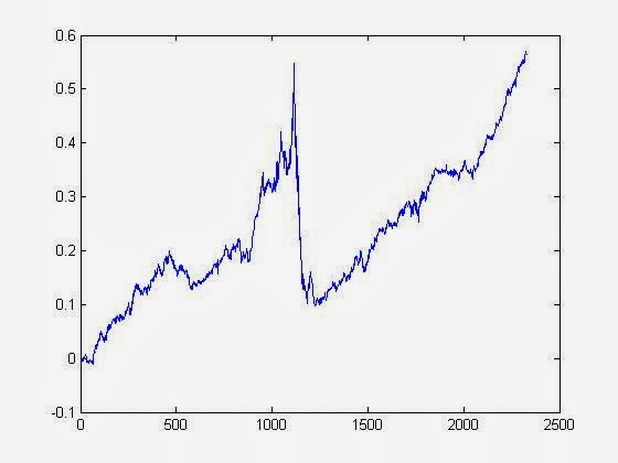
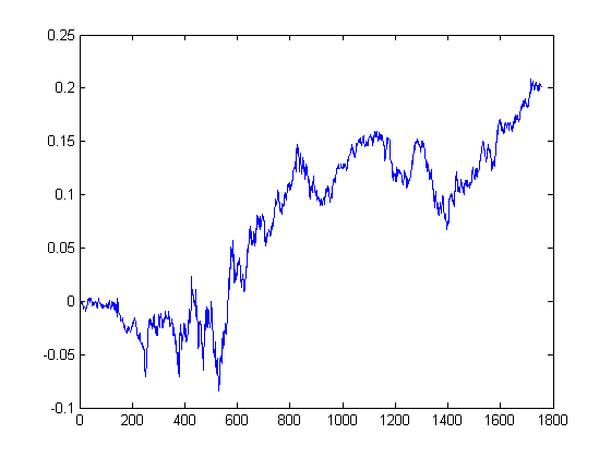
First, let's look at the Diversified Trends Indicator (formerly the S&P DTI index), which is a fairly generic trend-following strategy applied to futures. Here are the index values since inception (click to enlarge):

and here are the values for 2013:

After suffering relentless decline since 2009, it has finally shown positive returns YTD!

Now look at a momentum strategy on the soybean futures (ZS) that I have been working on. Here are the cumulative returns from 2009 to 2011 June:

and here the cumulative returns since then:

The difference is stark!

Despite evidences that indeed momentum strategies have enjoyed a general recovery, we must play the part of skeptical financial scientists and look for alternative theories. If any reader can tell us an alternative, plausible explanation why ZS should start to display trending behavior since July 2011, but not before, please post that in the comment area. The prize for the best explanation: I will disclose in private more details about this strategy to that reader. (To claim the prize, please include the last 4 digit of your phone number in the post for identification purpose.)

===
Upcoming events:

I will be teaching an online workshop on Momentum Strategies from July 30 - August 1. Registration info can be found here.
My friend Dr. Haksun Li is offering a Certificate in Quantitative Investment series of courses.

By Azouz Gmach

VIX Futures & Options are one of the most actively traded index derivatives series on the Chicago Board Options Exchange (CBOE). These derivatives are written on S&P 500 volatility index and their popularity has made volatility a widely accepted asset class for trading, diversifying and hedging instrument since their launch. VIX Futures started trading on March 26^th, 2004 on CFE (CBOE Future Exchange) and VIX Options were introduced on Feb 24^th, 2006.

VIX Futures & Options

VIX (Volatility Index) or the ‘Fear Index’ is based on the S&P 500 options volatility. Spot VIX can be defined as square root of 30 day variance swap of S&P 500 index (SPX) or in simple terms it is the 30-day average implied volatility of S&P 500 index options. The VIX F&O are based on this spot VIX and is similar to the equity indexes in general modus operandi. But structurally they have far more differences than similarities. While, in case of equity indices (for example SPX), the index is a weighted average of the components, in case of the VIX it is sum of squares of the components. This non-linear relationship makes the spot VIX non-tradable but at the same time the derivatives of spot VIX are tradable. This can be better understood with the analogy of Interest Rate Derivatives. The derivatives based on the interest rates are traded worldwide but the underlying asset: interest rate itself cannot be traded.

The different relation between the VIX derivatives and the underlying VIX makes it unique in the sense that the overall behavior of the instruments and their pricing is quite different from the equity index derivatives. This also makes the pricing of VIX F&O a complicated process. A proper statistical approach incorporating the various aspects like the strength of trend, mean reversion and volatility etc. is needed for modeling the pricing and behavior of VIX derivatives.

Research on Pricing Models

There has been a lot of research in deriving models for the VIX F&O pricing based on different approaches. These models have their own merits and demerits and it becomes a tough decision to decide on the most optimum model. In this regards, I find the work of Mr. Qunfang Bao titled ‘Mean-Reverting Logarithmic Modeling of VIX’quite interesting. In his research, Bao not only revisits the existing models and work by other prominent researchers but also comes out with suggestive models after a careful observation of the limitations of the already proposed models. The basic thesis of Bao’s work involves mean-reverting logarithmic dynamics as an essential aspect of Spot VIX.

VIX F&O contracts don’t necessarily track the underlying in the same way in which equity futures track their indices. VIX Futures have a dynamic relationship with the VIX index and do not exactly follow its index. This correlation is weaker and evolves over time. Close to expiration, the correlation improves and the futures might move in sync with the index. On the other hand VIX Options are more related to the futures and can be priced off the VIX futures in a much better way than the VIX index itself.

Pricing Models

As a volatility index, VIX shares the properties of mean reversion, large upward jumps & stochastic volatility (aka stochastic vol-of-vol). A good model is expected to take into consideration, most of these factors.

There are roughly two categories of approaches for VIX modeling. One is the Consistent approach and the other being Standalone approach.

I. Consistent Approach: - This is the pure diffusion model wherein the inherent relationship between S&P 500 & VIX is used in deriving the expression for spot VIX which by definition is square root of forward realized variance of SPX.

II. Standalone Approach: - In this approach, the VIX dynamics are directly specified and thus the VIX derivatives can be priced in a much simpler way. This approach only focuses on pricing derivatives written on VIX index without considering SPX option.

Bao in his paper mentions that the standalone approach is comparatively better and simpler than the consistent approach.

MRLR model

The most widely proposed model under the standalone approach is MRLR (Mean Reverting Logarithmic Model) model which assumes that the spot VIX follows a Geometric Brownian motion process. The MRLR model fits well for VIX Future pricing but appears to be unsuited for the VIX Options pricing because of the fact that this model generates no skew for VIX option. In contrast, this model is a good model for VIX futures.

MRLRJ model

Since the MRLR model is unable to produce implied volatility skew for VIX options, Bao further tries to modify the MRLR model by adding jump into the mean reverting logarithmic dynamics obtaining the Mean Reverting Logarithmic Jump Model (MRLRJ). By adding upward jump into spot VIX, this model is able to capture the positive skew observed in VIX options market.

MRLRSV model

Another way in which the implied volatility skew can be produced for VIX Options is by including stochastic volatility into the spot VIX dynamics. This model of Mean Reverting Logarithmic model with stochastic volatility (MRLRSV) is based on the aforesaid process of skew appropriation.

Both, MRLRJ and MRLRSV models perform equally well in appropriating positive skew observed in case of VIX options.

MRLRSVJ model

Bao further combines the MRLRJ and MRLRSV models together to form MRLRSVJ model. He mentions that this combined model becomes somewhat complicated and in return adds little value to the MRLRJ or MRLRSV models. Also extra parameters are needed to be estimated in case of MRLRSVJ model.

MRLRJ & MRLRSV models serve better than the other models that have been proposed for pricing the VIX F&O. Bao in his paper, additionally derives and calibrates the mathematical expressions for the models he proposes and derives the hedging strategies based on these models as well. Quantifying the Volatility skew has been an active area of interest for researchers and this research paper addresses the same in a very scientific way, keeping in view the convexity adjustments, future correlation and numerical analysis of the models etc. While further validation and back testing of the models may be required, but Bao’s work definitely answers a lot of anomalous features of the VIX and its derivatives.

---
Azouz Gmach works for QuantShare, a technical/fundamental analysis software.

===
My online Mean Reversion Strategies workshop will be offered in September. Please visit epchan.com/my-workshops for registration details.

Also, I will be teaching a new course Millisecond Frequency Trading (MFT) in London this October.

-Ernie

Can short-term price movement be predicted? (I am speaking of seconds or minutes here.) This is a question not only relevant to high frequency traders, but to every long-term investor as well. Even if one plans to buy and hold a stock for years, nobody likes to suffer short-term negative P&L immediately after entry into position.

One short-term prediction method that has long found favor with academic researchers and traders alike is order flow. Order flow is just signed transaction volume: if a transaction of 100 shares is classified as a "buy", the order flow is +100; if it is classified as a "sell", the order flow is -100. This might strike some as rather strange: every transaction has a buyer and seller, so what does it mean by a "buy" or a "sell"? Well, the "buyer" is defined as the one who is the "aggressor", i.e. one that is using a market order to buy at the ask price. (And vice versa for the seller, whom I will henceforth omit in this discussion.) The intuitive reason why a series of large "buy" market orders are predictive of short-term price increase is that if someone is so eager to go long, s/he is likely to know something about the market that others don't (either due to superior fundamental knowledge or technical model), so we better join her/him! Such superior traders are often called "informed traders", and their order flow is often called "toxic flow". Toxic, that is, to the uninformed market maker.

In theory, if one has a tick data feed, one can tell whether an execution is a "buy" or "sell" by comparing the trade price with the bid and ask price: if the trade price is equal to the ask, it is a "buy". This is called the "Quote Rule". But in practice, there is a hitch. If the bid and ask prices change quickly, a buy market order may end up buying at the bid price if the market has fortuitously moved lower since the order was sent. Besides, perhaps 1/3 of trading in the US equities markets take place in dark pools or via hidden orders, so the quotes are simply invisible and order flow non-computable. So this classification scheme is not foolproof. Therefore, a number of researchers (see "Flow Toxicity and Volatility in a High Frequency World" by Easley, et. al.) proposed an alternative, "easier", method to compute order flow. Instead of checking the trade price of each tick, they just need the "open" and "close" trade prices of a bar, preferably a volume bar, and assign a fraction of the volume in that bar to "buy" or "sell" depending on whether the close price is higher or lower than the open price. (The assignment formula is based on the cumulative probability density of a Gaussian distribution, which incidentally models price changes of volume bars, but not time bars, pretty well.) The absolute difference between buy and sell volume expressed as a fraction of the total volume is called "VPIN" by the authors, or Volume-Synchronized Probability of Informed Trading. The higher VPIN is, the more likely we will experience short-term momentum due to informed trading.

Theory and intuition aside, how well does order flow work in practice as a short-term predictor in various markets? And how predictive is VPIN as compared to the old Quote Rule? In my experience, while this indicator is predictive of price change, the change is often too small to overcome transaction costs including the bid-ask spread. And more disturbingly, in those markets where both Quote Rule and VPIN should work (e.g. futures markets), VPIN has so far underperformed Quote Rule, despite (?) it being patented and highly touted. I have informally polled other investment professionals on their experience, and the answer usually come back indifferent as well.

Do you have live experience with VPIN? Or more generally, do you find strategies built using volume bars superior to those using time bars? If so, please leave us your comments!

===

My online Quantitative Momentum Strategies workshop will be offered in December. Please visit epchan.com/my-workshops for registration details.

In my recent book, I highlighted a difference between cointegration (pair) trading of price spreads and log price spreads. Suppose the price spread hA*yA-hB*yB of two stocks A and B is stationary. We should just keep the number of shares of stocks A and B fixed, in the ratio hA:hB, and short this spread when it is much higher than average, and long this spread when it is much lower. On the other hand, for a stationary log price spread hA*log(yA)-hB*log(yB), we need to keep the market values of stocks A and B fixed, in the ratio hA:hB, which means that at the end of every bar, we need to rebalance the shares of A and B due to price changes.

For most cointegrating pairs that I have studied, both the price spreads and the log price spreads are stationary, so it doesn't matter which one we use for our trading strategy. However, for an unusual pair where its log price spread cointegrates but price spread does not (Hat tip: Adam G. for drawing my attention to one such example), the implication is quite significant. A stationary price spread means that prices differences are mean-reverting, a stationary log price spread means that returns differences are mean-reverting. For example, if stock A typically grows 2 times as fast as B, but has been growing 2.5 times as fast recently, we can expect the growth rate differential to decrease going forward. We would still short A and long B, but we would exit this position when the growth rates of A vs B return to a 2:1 ratio, and not when the price spread of A vs B returns to a historical mean. In fact, the price spread of A vs B should continue to increase over the long term.

This much is easy to understand. But thanks to a reader Ferenc F. who referred me to a paper by Fernholz and Maguire, I realize there is a simple mathematical relationship between stock A and B in order for their log prices to cointegrate.

Let us start with a formula derived by these authors for the change in log market value P of a portfolio of 2 stocks: d(logP) = hA*d(log(yA))+hB*d(log(yB))+gamma*dt.

The gamma in this equation is

gamma=1/2*(hA*varA + hB*varB), where varA is the variance of stock A minus the variance of the portfolio market value, and ditto for varB.

Note that this formula holds for a portfolio of any two stocks, not just when they are cointegrating. But if they are in fact cointegrating, and if hA and hB are the weights which create the stationary portfolio P, we know that d(logP) cannot have a non-zero long term drift term represented by gamma*dt. So gamma must be zero. Now in order for gamma to be zero, the covariance of the two stocks must be positive (no surprise here) and equal to the average of the variances of the two stocks. I invite the reader to verify this conclusion by expressing the variance of the portfolio market value in terms of the variances of the individual stocks and their covariance, and also to extend it to a portfolio with N stocks. This cointegration test for log prices is certainly simpler than the usual CADF or Johansen tests! (The price to pay for this simplicity? We must assume normal distributions of returns.)

===

My online Quantitative Momentum Strategies workshop will be offered on December 2-4. Please visit epchan.com/my-workshops for registration details.

Folklore has it that VIX is a reasonable leading indicator of risk. Presumably that means if VIX is high, then there is a good chance that the future return of the SP500 will be negative. While I have found some evidence that this is true when VIX is particularly elevated, say above 30, I don't know if anyone has established a negative correlation between VIX and future returns. (Contemporaneous VIX and SP500 levels do have a very nice linear relationship with negative slope.)

Interestingly, the situation is much clearer if we examine the Variance Risk Premium (VRP), which is defined as the difference between a model-free implied volatility (of which VIX is the most famous example) and the historical volatility over a recent period. The relationship between VRP and future returns is examined in a paper by Chevallier and Sevi in the context of OVX, which is the CBOE Crude Oil Volatility Index. They have found that there is a statistically significant negative linear relationship between VRP and future 1-month crude oil futures (CL) returns. The historical volatility is computed over 5-minute returns of the most recent trading day. (Why 5 minutes? Apparently this is long enough to avoid the artifactual volatility induced by bid-ask bounce, and short enough to truly sample intraday volatility.) If you believe in the prescience of options traders, it should not surprise you that the regression coefficient is negative (i.e. a high VRP predicts a lower future return).

I have tested a simple trading strategy based on this linear relationship. Instead of using monthly returns, I use VRP to predict daily returns of CL. It is very similar to a mean-reverting Bollinger band strategy, except that here the "Bollinger bands" are constructed out of moving first and third quartiles of VRP with a 90-day lookback. Given that VRP is far from normally distributed, I thought it is more sensible to use quartiles rather than standard deviations to define the Bollinger bands. So we buy a front contract of CL and hold for just 1 day if VRP is below its moving first quartile, and short if VRP is above its moving third quartile. It gives a decent average annual return of 17%, but performance was poor in 2013.

Naturally, one can try this simple trading strategy on the E-mini SP500 future ES also. This time, VRP is VIX minus the historical volatility of ES. Contrary to folklore, I find that if we regress the future 1 day ES return against VRP, the regression coefficient is positive. This means that an increase of VIX relative to historical volatility actually predicts an increase in ES! (Does this mean investors are overpaying for put options on SPX for portfolio protection?) Indeed, the opposite trading rules from the above give positive returns: we should buy ES if VRP is above its moving third quartile, and short ES if VRP is below its moving first quartile. The annualized return is 6%, but performance in 2013 was also poor.

As the authors of the paper noted, whether or not VRP is a strong enough stand-alone predictor of returns, it is probably useful as an additional factor in a multi-factor model for CL and ES. If any reader know of other volatility index like VIX and OVX, please do share with us in the comments section!

===

My online Backtesting Workshop will be offered on February 18-19. Please visit epchan.com/my-workshops for registration details. Furthermore, I will be teaching my Mean Reversion, Momentum, and Millisecond Frequency Trading workshops in London on March 17-21, and in Hong Kong on June 17-20.

Contrary to my tradition of alerting readers to new and fancypants factors for predicting stock returns (while not necessarily endorsing any of them), I report that Lyle and Wang have recently published new research demonstrating the power of two very familiar factors: book-to-market ratio (BM) and return-on-equity (ROE).

The model is simple: at the end of each calendar quarter, compute the log of BM and ROE for every stock based on the most recent earnings announcement, and regress the next-quarter return against these two factors. One subtlety of this regression is that the factor loadings (log BM and ROE) and the future returns for stocks within an industry group are pooled together. This makes for a cross-sectional factor model, since the factor loadings (log BM and ROE) vary by stock but the factor returns (the regression coefficients) are the same for all stocks within an industry group. (A clear elucidation of cross-sectional vs time-series factor models can be found in Section 17.5 of Ruppert.) If we long stocks within the top decile of expected returns and short the bottom decile and hold for a quarter, the expected annualized average returns of this model is an eye-popping 26% or so.

I have tried to replicate these results, but unfortunately I couldn't. (My program generated a measly, though positive, APR.) The data requirement and the program are both quite demanding. I am unable to obtain the 60 quarters of fundamental data that the authors recommended - I merely have 40. I used the 65 industry groups defined by the GIC industry classifications, while the authors used the 48 Fama-French industry groups. Finally, I am unsure how to deal with stocks which have negative book values or earnings, so I omit those quarterly data. If any of our readers are able to replicate these results, please do let us know.

The authors and I used Compustat database for the fundamental data. If you do not have subscription to this database, you can consider a new, free, website called Thinknum.com. This website makes available all data extracted from companies' SEC filings starting in 2009 (2011 for small caps). There is also a neat integration with R described here.

*** Update ***

I forgot to point out one essential difference between the method in the cited paper and my own effort: the paper used the entire stock universe except for stocks cheaper than $1, while I did my research only on SP500 stocks (Hat tip to Prof. Lyle who clarified this). This turns out to be of major importance: a to-be-published paper by our reader I. Kaplan reached the conclusion that "Linear models based on value factors do not predict future returns for the S&P 500 universe for the past fifteen years (from 1998 to 2013)."

===

Speaking of new trading technology platforms that provide historical data for backtesting (other than Thinknum.com and the previously mentioned Quantopian.com), here is another interesting one: QuantGo.com. It provides institutional intraday historical data through its data partners from 1 minute bars to full depth of book in your own private cloud running on Amazon EC2 account for a low monthly rate. They give unlimited access to years of historical data for a monthly data access fee, for examples US equities Trades and Quotes (TAQ) for an unlimited number of years are $250 per month of account rental, OPRA TAQ $250 permonth and tagged news is $200. Subscribers control and manage their own computer instances, so can install and use whatever software they want on them to backtest or trade using the data. The only hitch is that you are not allowed to download the vendor data to your own computer, it has to stay in the private cloud.

===

Follow @chanep to receive my occasional tweets on interesting quant trading industry news and articles.

===

My online Mean Reversion Strategies Workshop will be offered on April 1-3. Please visit epchan.com/my-workshops for registration details. Furthermore, I will be teaching my Mean Reversion, Momentum, and Millisecond Frequency Trading workshops in London on March 17-21, and in Hong Kong on June 17-20.

In my last post, I reported that the fundamental factors used by Lyle and Wang seem to generate no returns on SP500 large cap stocks. These fundamental factors are the growth factor return-on-equity (ROE), and the value factor book-to-market ratio (BM).

I have since studied the effect of these factors on SP600 small cap stocks since 2004, using a survivorship-bias-free database combining information from both Compustat and CRSP. This time, the factors do produce an annualized average return of 4.7% and a Sharpe ratio of 0.8. Though these numbers are nowhere near the 26% return that Lyle and Wang found, they are still statistically significant. I have plotted the equity curve below.

Equity curve of long-short small-cap portfolio based on regression on ROE and BM factors (2004-2013)

One may wonder whether ROE or BM is the more important factor. So I run a simpler model which uses one factor at a time to rank stocks every day. We buy stocks in top decile of ROE, and short the ones in the bottom decile. Ditto for BM. I found an annualized average return of 5% with a Sharpe ratio of 0.8 using ROE only, and only 0.8% with a Sharpe ratio of 0.09 using BM only. The value factor BM is almost completely useless! Indeed, if we were to first sort on ROE, pick the top and bottom deciles, and then sort on BM, and pick the top and bottom halves, the resulting average return is almost the same as sorting on ROE alone. I plotted the equity curve for sorting on ROE below.

Equity curve of long-short small-cap portfolio based on top and bottom deciles of ROE (2004-2013)

Notice the sharp drawdown from 2008-05-30 to 2008-11-04, and the almost perfect recovery since then. This mirrors the behavior of the equity market itself, which raises the question of why we bother to construct a long-short portfolio at all as it provides no hedge against the downturn. It is also interesting to note that this factor does not exhibit "momentum crash" as explained in a previous article: it does not suffer at all during the market recovery. This means we should not automatically think of a fundamental growth factor as similar to price momentum.

My conclusion was partly corroborated by I. Kaplan who has written a preprint on a similar topic. He found that a long-short portfolio created using the ratio EBITA/Enterprise Value on large caps generates a Sharpe ratio of about 0.6 but with very little drawdown unlike the ROE factor that I studied above as applied to small caps.

As Mr. Kaplan noted, these results are in some contradiction not only with Lyle and Wang's paper, but also with the widely circulated paper by Cliff Asness et al. These authors found the the BM factor works in practically every asset class. Of course, the timeframe of their research is much longer than my focus above. Furthermore, they have excluded financial and penny stocks, though I did not find such restrictions to have great impact in my study of large cap portfolios. In place of a fundamental growth factor, these authors simply used price momentum over an 11-month period (skipping the most recent month), and found that this is also predictive of future quarterly returns.

Finally, we should note that the ROE and BM factors here are quite similar to the Return-on-Capital and Earnings Yield factors used by Joel Greenblatt in his famous "Little Book That Still Beats The Market". One wonders if those factors suffer a similar drawdown during the financial crisis.

===

My online Momentum Workshop will be offered on May 5-7. Please visit epchan.com/my-workshops for registration details. Furthermore, I will be teaching my Mean Reversion, Momentum, and Millisecond Frequency Trading workshops in Hong Kong on June 17-20.

Readers of zerohedge.com will no doubt be impressed by this chart and the accompanying article:

Cumulative returns of most shorted stocks relative to SPX

Cumulative Returns of Most Shorted Stocks in 2013

Indeed, short interest (expressed as the number of shares shorted divided by the total number of shares outstanding) has long been thought to be a useful factor. To me, the counter-intuitive wisdom is that the more a stock is shorted, the better is its performance. You might explain that by saying this is a result of the "short squeeze", when there is jump in price perhaps due to news and stock lenders are eager to sell the stock they own. If you have borrowed this stock to short, your borrowed stock may be recalled and you will be forced to buy cover at this most inopportune time. But this is an unsatisfactory explanation, as this will result only in a short term (upward) momentum in price, not the sustained out-performance of the most shorted stocks. This long-term out-performance seems to suggest that short sellers are less informed than the average trader, which is odd.

Whatever the explanation, I am intrigued to find out if short interest really is a good factor to incorporate into a comprehensive factor model over the long term.

The result? Not particularly impressive. It turns out that 2013 was one of the best years for this factor (hence the impressive chart above). For that year, a daily-rebalanced long-short portfolio (long 50 most shorted stocks and short 50 least shorted stocks in the SPX) returned 6.9%, with a Sharpe ratio of 2 and a Calmar ratio of 2.9. However, if we extend our backtest to 2007, the APR is only 2.8%, with a Sharpe ratio of 0.5 and a Calmar ratio of 0.3. This backtest was done using survivorship-bias-free data from CRSP, with short interest data provided by Compustat.

Here is the cumulative returns chart from 2007-2013:

Cumulative Returns of LS Portfolio based on Short Interest: 2007-2013

Interesting, trying this on the SP600 small-cap universe yielded negative returns, possibly meaning that short-sellers of small caps do have superior information.

I promise, this will be the last time I talk about factors in a while!

===
Tech Update:

I was shocked to learn that Matlab now offers licenses for just $149 - the so-called Matlab Home (h/t: Ken H.) In addition, its Trading Toolbox now offers API connection to Interactive Brokers, in addition to a few other brokerages. I am familiar with both Matlab and R, and while I am impressed by the large number of free, sophisticated statistical packages in R, I still stand by Matlab as the most productive platform for developing our own strategies. The Matlab development (debugging) environment is just that much more polished and easy-to-use. The difference is bigger than Microsoft Word vs. Google Docs.

A reader Ravi B. told me that there is a website called www.seasonalgo.com if you want to try out different seasonal futures strategies.

Finally, a startup at inovancetech.com offers machine learning algorithms to help you find the best combination of technical indicators for trading FX.

===
Workshops Update:

I am now offering the Millisecond Frequency Trading (MFT) Workshop as an online course on June 26- 27. Previously, I have only offered it live in London and to a few institutional investors. It has two main parts:

Part 1: introducing techniques for traders who want to avoid HFT predators.

Part 2: how to backtest a strategy that requires tick data with millisecond resolution using Matlab.

The example strategy used is based on order flow. For more details, please visit epchan.com/my-workshops.

Additionally, I will be teaching the Mean Reversion and Momentum (but not MFT) workshops in Hong Kong on June 17-20.

Extracting roll returns from futures

An options workshop and other miscellany

Order flow as a predictor of return

A leveraged ETFs strategy

The Importance of 2 (as Sharpe Ratio)

The Pseudo-science of Hypothesis Testing

A stock factor based on option volatility smirk

A workshop, a webinar, and a question

What Can Quant Traders Learn from Taleb's "Antifragile"?

An Integrated Development Environment for High Frequency Strategies

Nonlinear Trading Strategies

My new book on Algorithmic Trading is out

Momentum Crash and Recovery

Guest Post: A qualitative review of VIX F&O pricing and hedging models

How Useful is Order Flow and VPIN?

Cointegration Trading with Log Prices vs. Prices

Variance Risk Premium for Return Forecasting

Fundamental factors revisited, with a technology update

Update on the fundamentals factors: their effect on small cap stocks

Short Interest as a Factor